Microbiota changes on the surface of pig carcasses during refrigerated transportation and marketing

Figures (5) Tables (1)

Figure 1.
A diagram of sampling sites for microbial counting.
Figure 2.
Changes in vehicle temperature and humidity and carcass temperature during transportation. (a) Vehicle temperature, (b) vehicle humidity, (c) carcass temperature.
Figure 3.
Microbial colony counts on the surface of pig carcasses. (a) Before transportation, (b) at the end point of transportation, (c−f) at the different market points. a,b Different letters indicate significant differences among groups (P < 0.05).
Figure 4.
PCA scores plot of samples. T_0km, the start point of transportation; T_200km-a, T_300km-a, T_400km-a, T_500km-a, the end points of 200, 300, 400 and 500 km transportation; T_200km-b, T_300km-b, T_400km-b, T_500km-b, the market points after 200, 300, 400, and 500 km transportation.
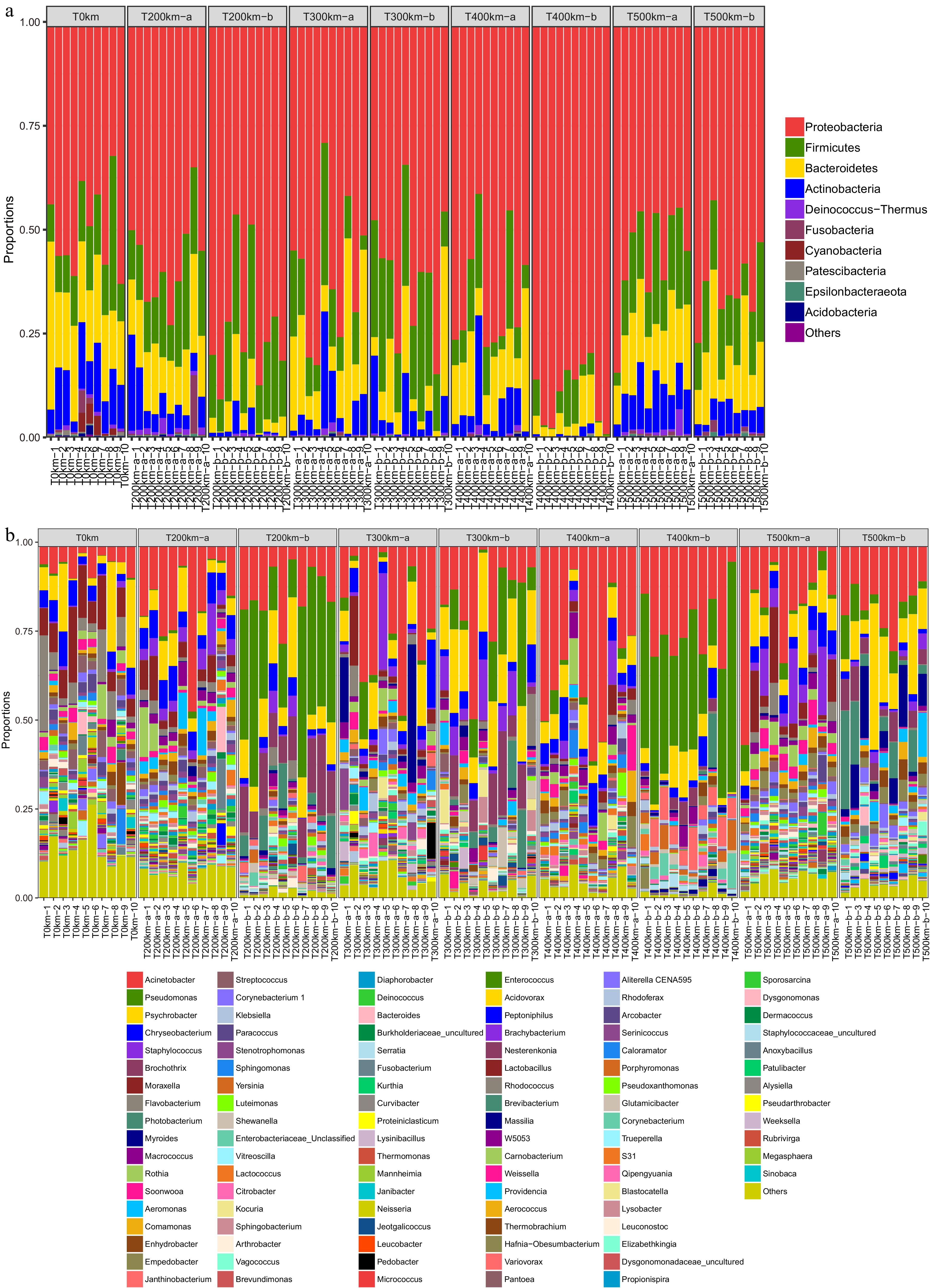
Figure 5.
Microbial composition in samples. (a) Phyla; (b) genera. T_0km, the start point of transportation; T_200km-a, T_300km-a, T_400km-a, T_500km-a, the end points of 200, 300, 400 and 500 km transportation; T_200km-b,T_300km-b, T_400km-b, T_500km-b, the market points after 200, 300, 400, and 500 km transportation.

Transportation distance /km	Vehicle temperature/ºC	Vehicle humidity/ºC	Carcass temperature/ºC
200	3.49 ± 0.21^ab	91.10 ± 9.87^a	2.87 ± 0.54^ab
300	3.42 ± 0.19^ab	88.83 ± 5.70^ab	3.04 ± 0.51^ab
400	3.34 ± 0.21^b	83.73 ± 5.26^b	2.70 ± 0.43^b
500	3.62 ± 0.21^a	88.16 ± 5.81^ab	3.25 ± 0.35^a
^a,b Different letters in the same column indicate significant differences among distance groups (P < 0.05).

Table 1.

Temperature and humidity values in refrigerated vehicles.