Performance and stability of yield in response to plant density, year and location in maize hybrids of Northwest China

Figures (4) Tables (2)

Figure 1.
Yield changes under different conditions. (a) Yield changes at different densities. (b) Yield changes among different locations at each density. (c) Yield changes among different years at the each density.
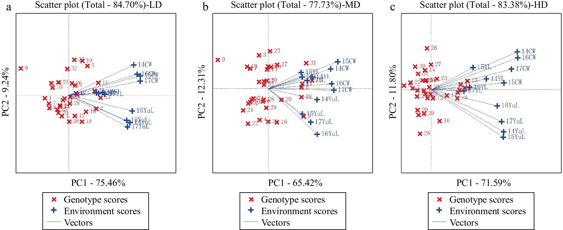
Figure 2.
Relationships between test environments at different densities.
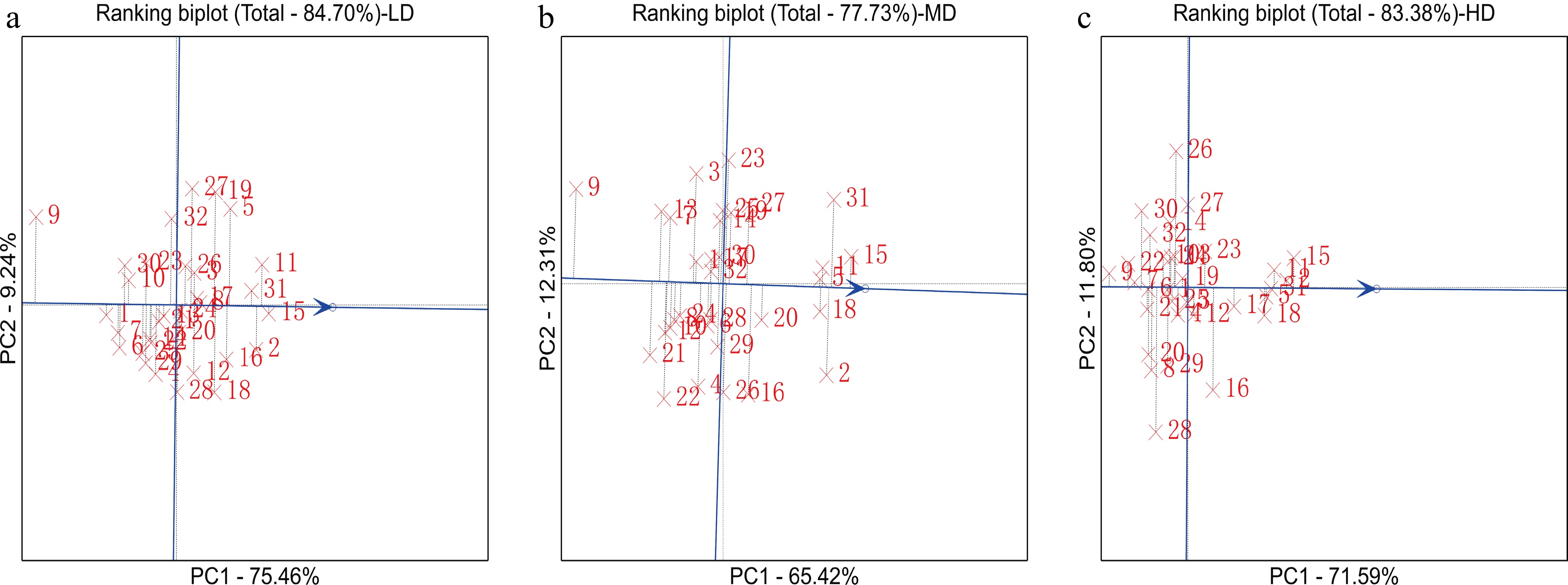
Figure 3.
GGE biplot for the grain yield of 32 hybrid combinations across 12 environments. From left to right, the graph shows the hybrid combinations with high yield and stability at LD, MD and HD. The data were not transformed (transform = 0), were not standardized (scale = 0), and were environment-centred (centring = 2). The biplot was created based on environment-focused singular value partitioning (SVP = 1) and is therefore appropriate for visualizing the relationships among genotypes.
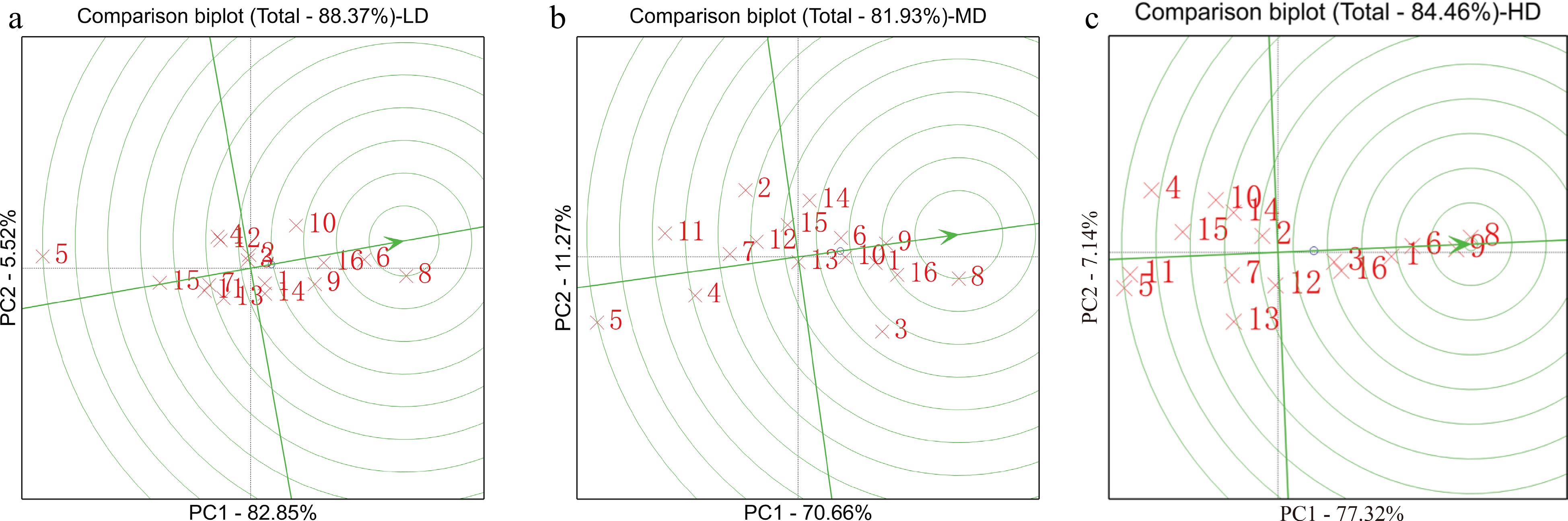
Figure 4.
GGE biplot for the GCA of 16 inbred lines across 12 environments. From left to right, the graph shows the high GCA and stability of inbred lines at LD, MD and HD. The parameters were not transformed (transform = 0), not standardized (scale = 0) and environment-centred (centring = 2). The biplot was created based on environment-focused singular value partitioning (SVP = 1) and is therefore appropriate for visualizing the relationships among genotypes. Understanding the genetic basis of inbred lines is crucial for appropriate breeding design.

Source of variation	d.f.	LD		MD		HD
Source of variation	d.f.	GY	PSQ(%)	GY	PSQ(%)	GY	PSQ(%)
Genotype (G)	31	18.80^**	20.41%	23.91^**	21.17%	33.01^**	26.20%
Environment (E)	11	173.74^**	66.94%	193.23^**	60.71%	193.09^**	54.38%
Location (L)	2	951.91^**	66.68%	979.09^**	55.93%	995.92^**	51.00%
Year (Y)	3	0.93^**	0.10%	23.34^**	2.00%	16.67^**	1.28%
Location × Year (L × Y)	6	0.75^**	0.16%	16.24^**	2.78%	13.70^**	2.10%
Genotype × Environment (G × E)	341	0.75^**	8.90%	1.36^**	13.20%	1.48^**	12.94%
Genotype × Location (G × L)	62	2.62^**	5.69%	3.96^**	7.01%	4.56^**	7.24%
Genotype × Year (G × Y)	93	0.38^**	1.24%	0.90^**	2.39%	0.73^**	1.75%
Genotype × Location × Year (G × L × Y)	186	0.30^**	1.97%	0.72^**	3.80%	0.83^**	3.96%
* and ** indicate significance at the 0.05 and 0.01 probability levels, respectively. GY: Grain yield; LD: 45,000 plants ha⁻¹; MD: 67,500 plants ha⁻¹; HD: 90,000 plants ha⁻¹; Rep: Repetition; PSQ: Percentage of the sum of squares.

Table 1.

Analysis of variance of grain yield under different densities.

Source of variation	d.f.	LD	MD	HD
GCA	15	23.02^**	26.37^**	39.54^**
SCA	15	15.83^**	22.96^**	24.94^**
GCA × L	30	1.65^**	3.58^**	3.69^**
GCA × Y	45	0.36^**	0.93^**	0.94^**
SCA × L	30	3.39^**	2.80^**	5.65^**
SCA × Y	45	0.32^**	0.71^**	0.53^**
GCA × L × Y	90	0.30^**	0.83^**	0.87^**
SCA × L × Y	90	0.29^**	0.56^**	0.80^**
Rep	2	0.001	0.37	3.28
Residual	766	0.14	0.22	0.32
* and ** indicate significance at the 0.05 and 0.01 probability levels, respectively; GCA: general combining ability; SCA: special combining ability; GCA × L: interaction of general combining ability and location; GCA × Y: interaction of general combining ability and year; SCA × L: interaction of special combining ability and location; SCA × Y: interaction of special combining ability and year; GCA × L × Y: interaction of general combining ability, location and year; SCA × L × L: interaction of special combining ability, location and year.

Table 2.

Analysis of variance of the combining ability of grain yield under different densities.