-
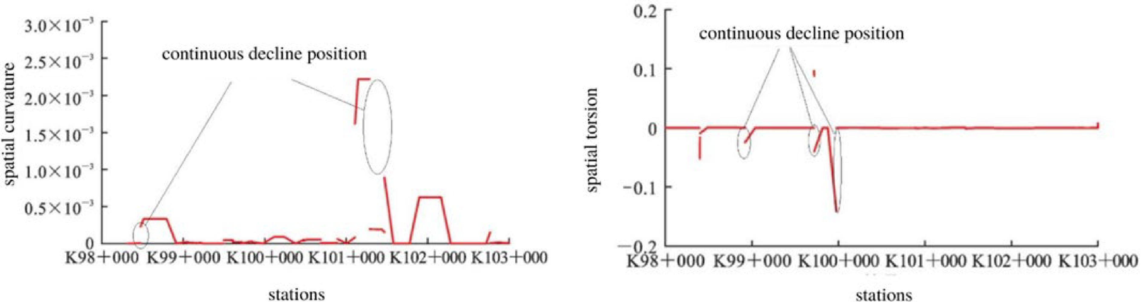
Figure 1.
Variation of curvature and torsion in Euclidean three-dimensional space.
-
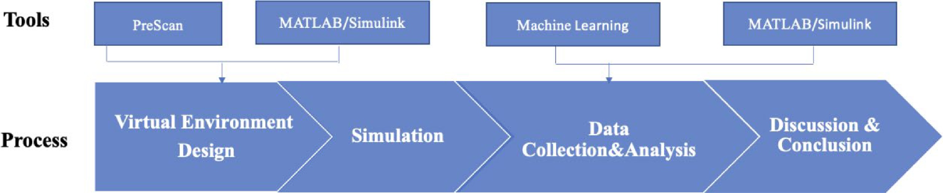
Figure 2.
Proposed pipeline for this study.
-
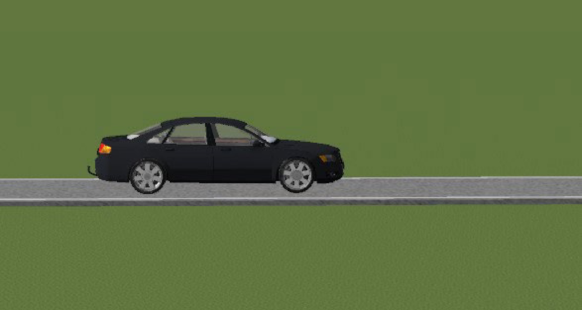
Figure 3.
Illustration of the vehicle used in this study.
-
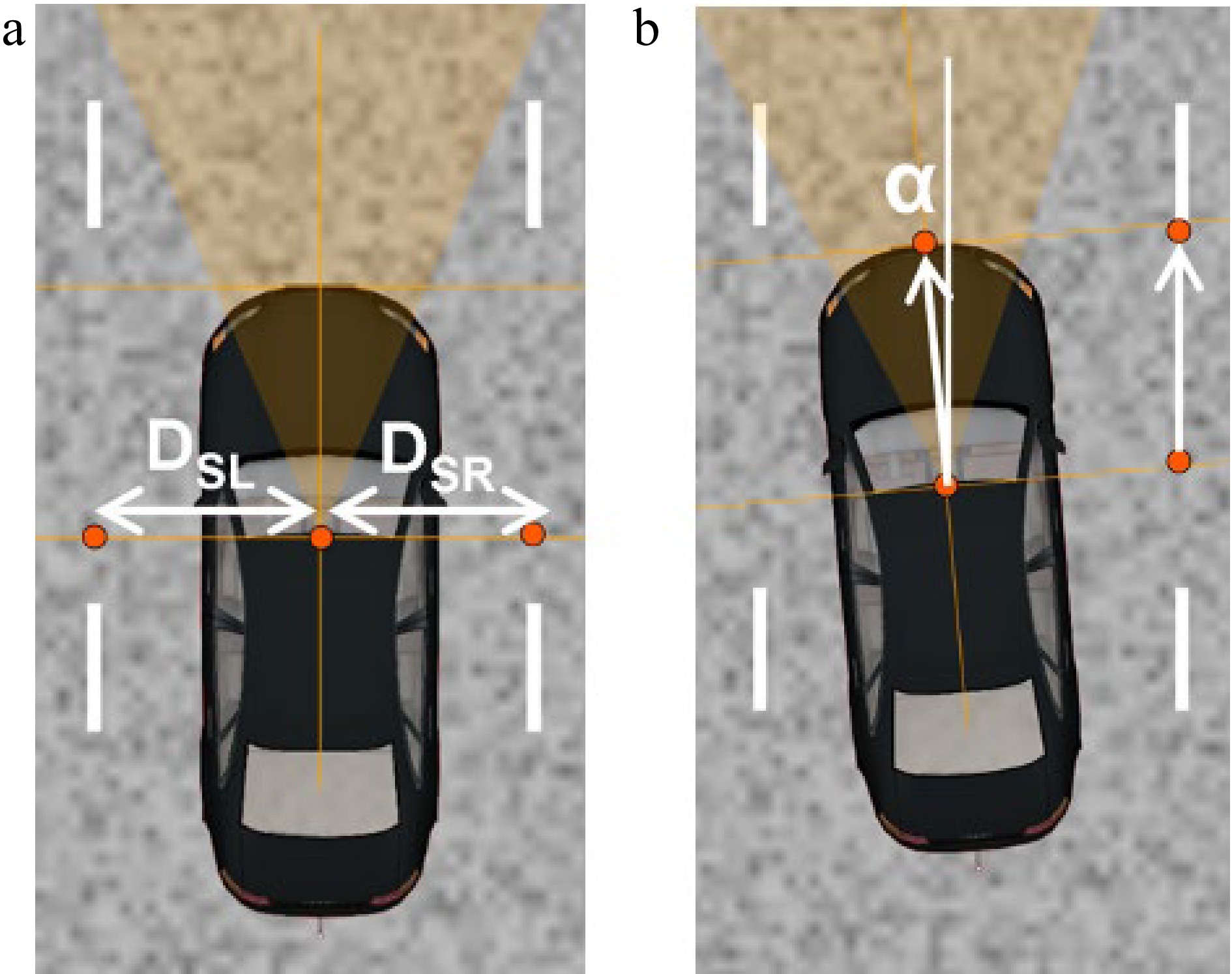
Figure 4.
Lane marker detection system. (a) Center line. (b) Angle DSL: Distance between the Sensor to the Left Line DRS: Distance between the Sensor to the Right Line α: the drift angle between sensor heading direction (= vehicle heading).
-
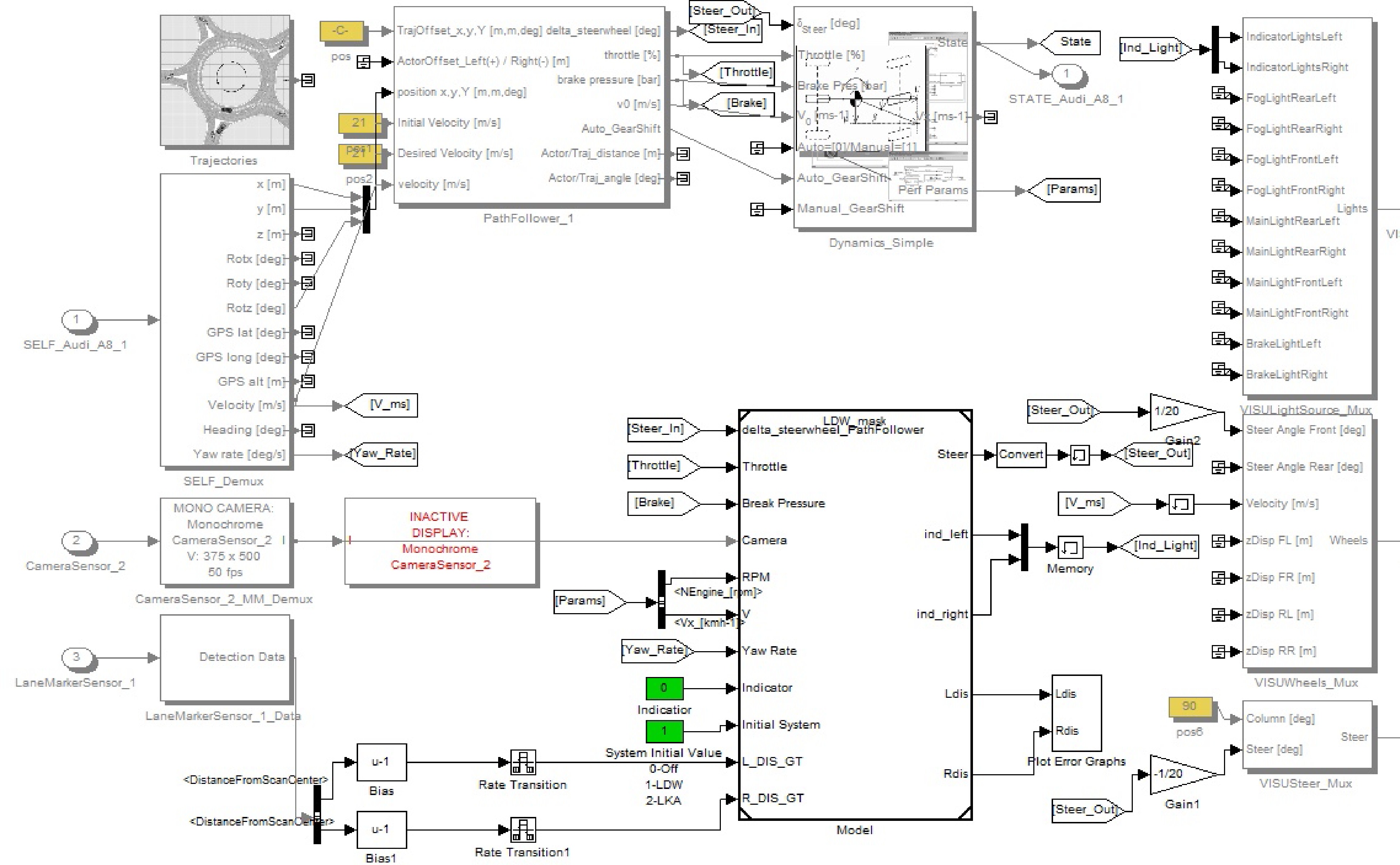
Figure 5.
LKAS controller with the visual features connections.
-
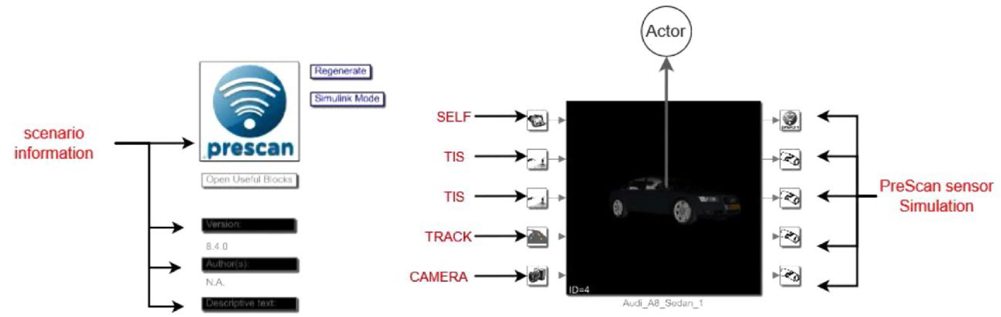
Figure 6.
Control system of infrastructure, actors, and sensors in MATLAB/Simulink.
-
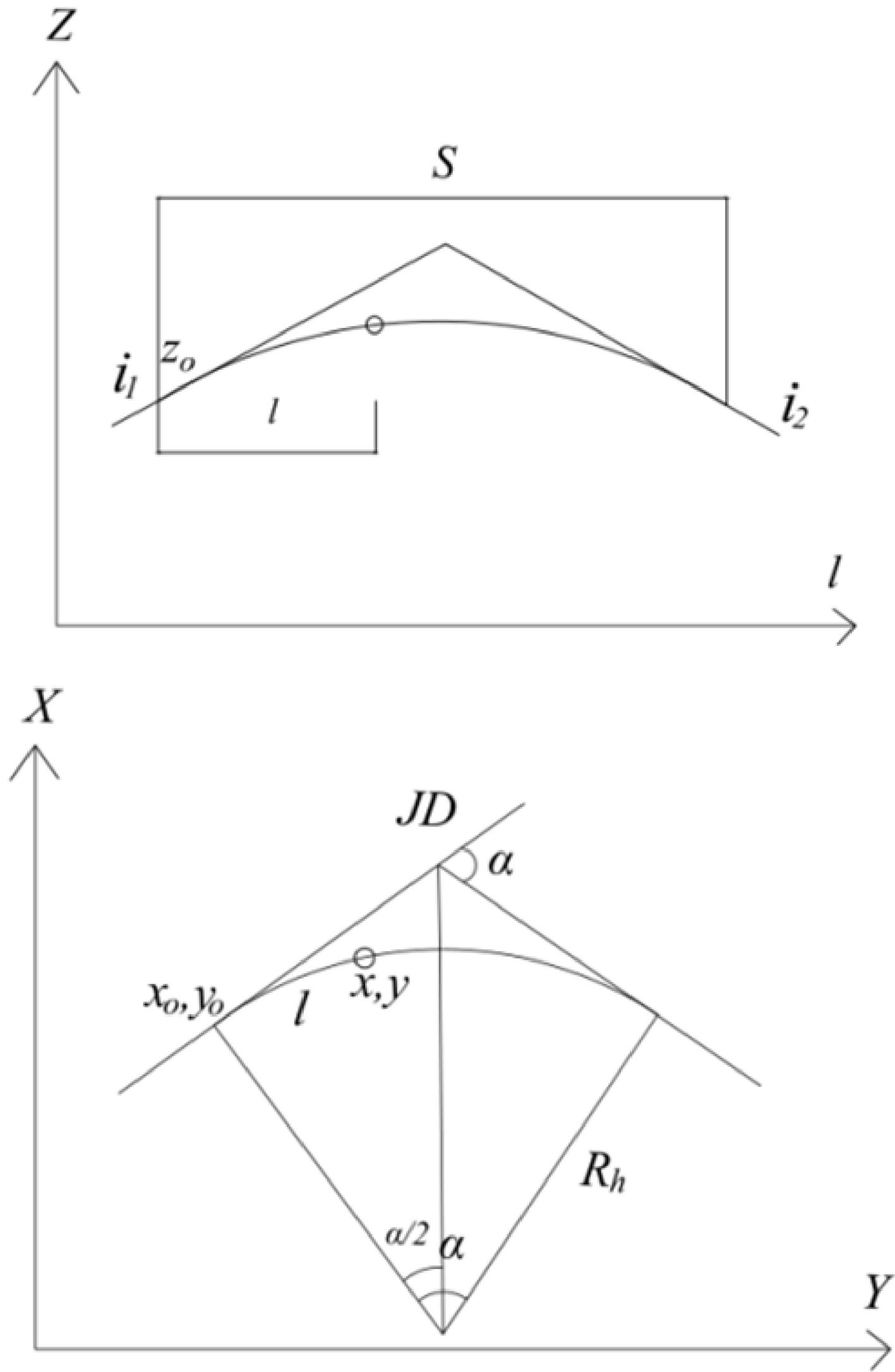
Figure 7.
Diagram of horizontal and vertical curve parameters.
-
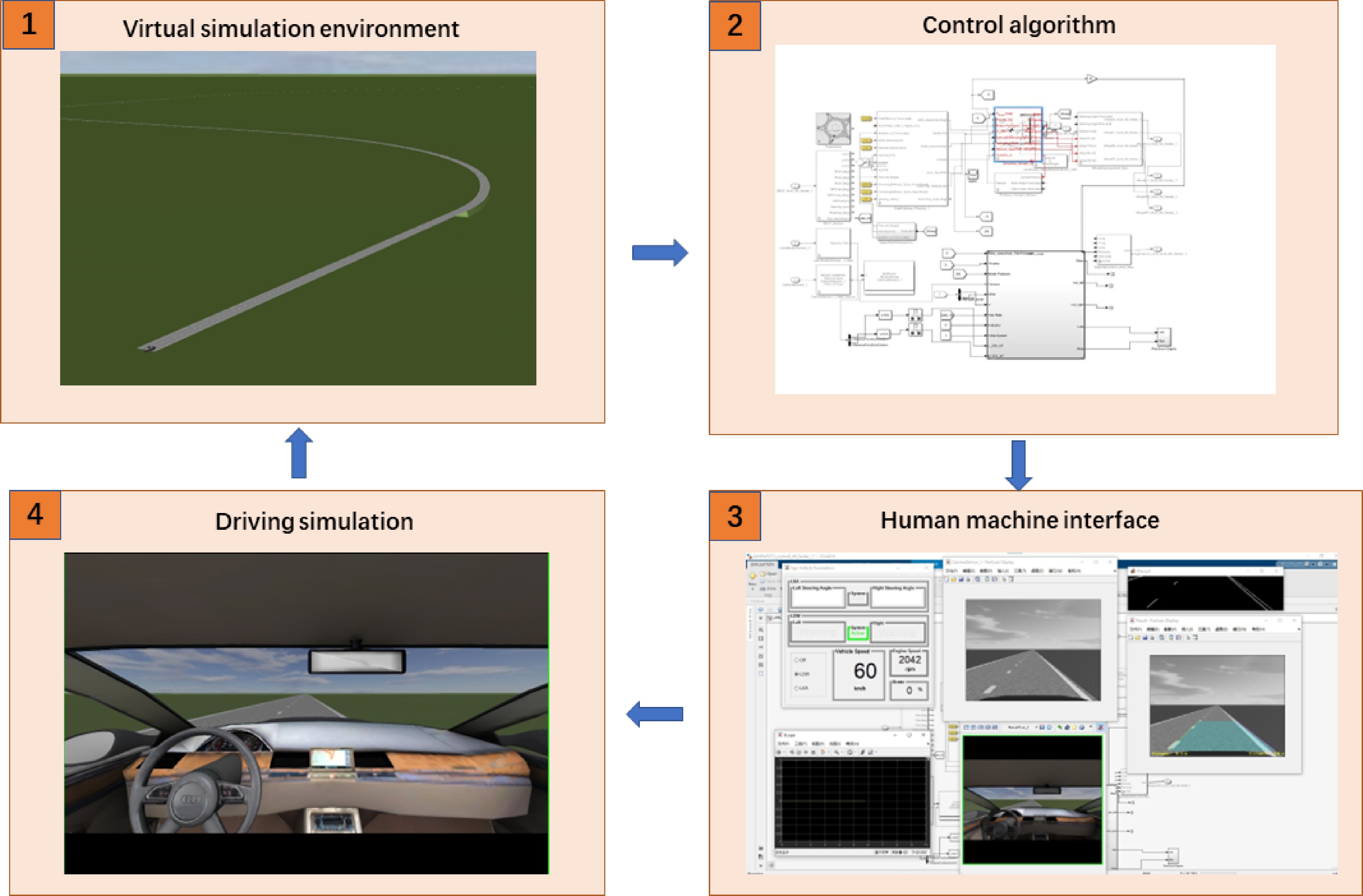
Figure 8.
Experimental process.
-
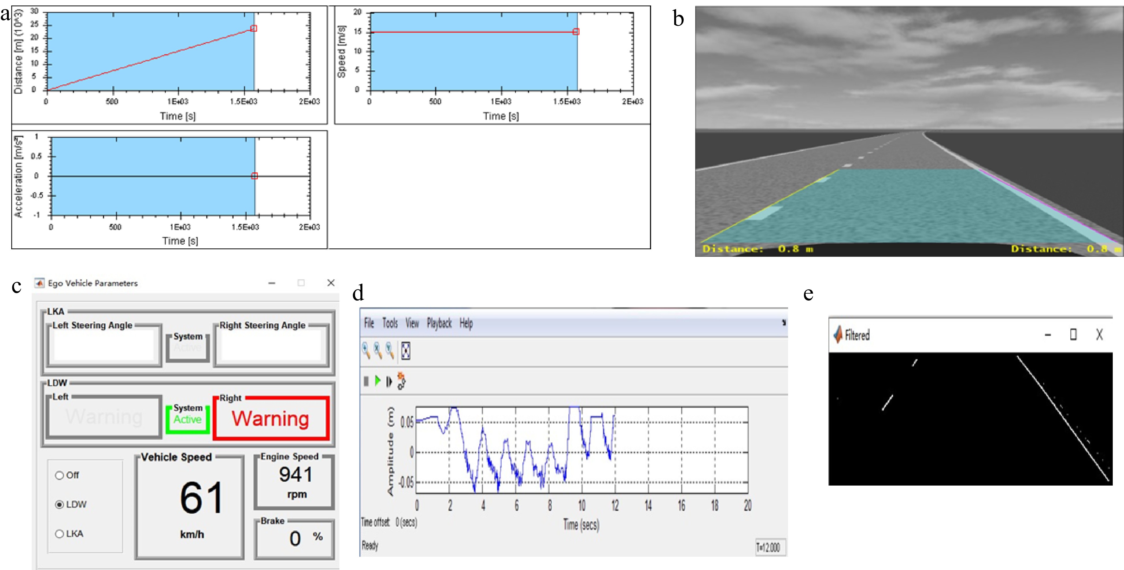
Figure 9.
Data visualization in Prescan. (a) Av speed and acceleration profile. (b) Camera sensor output. (c) Lane keeping assistant GUI. (d) Car to lane distance error. (e) Filtered image output.
-
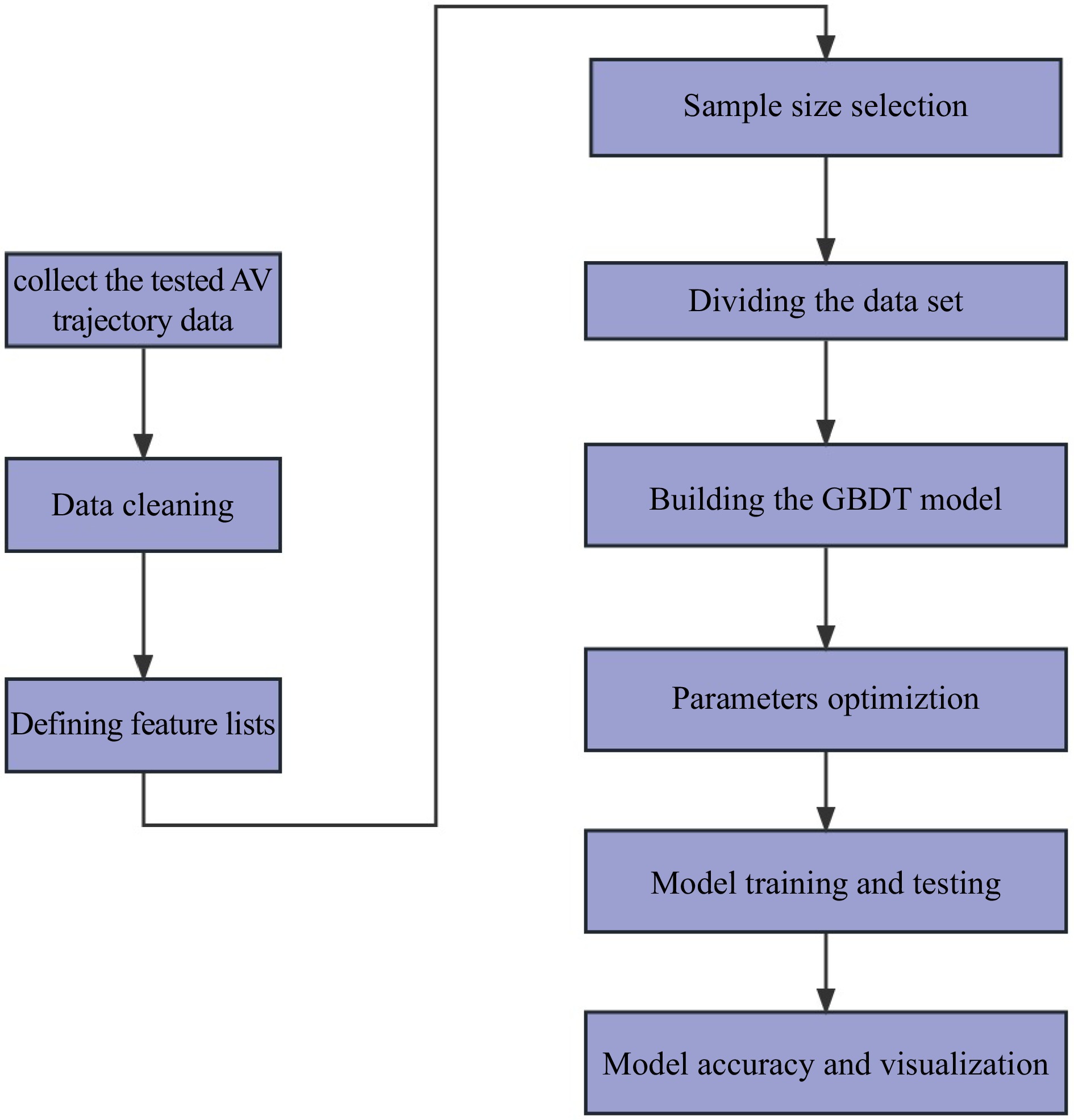
Figure 10.
GBDT model overall framework.
-
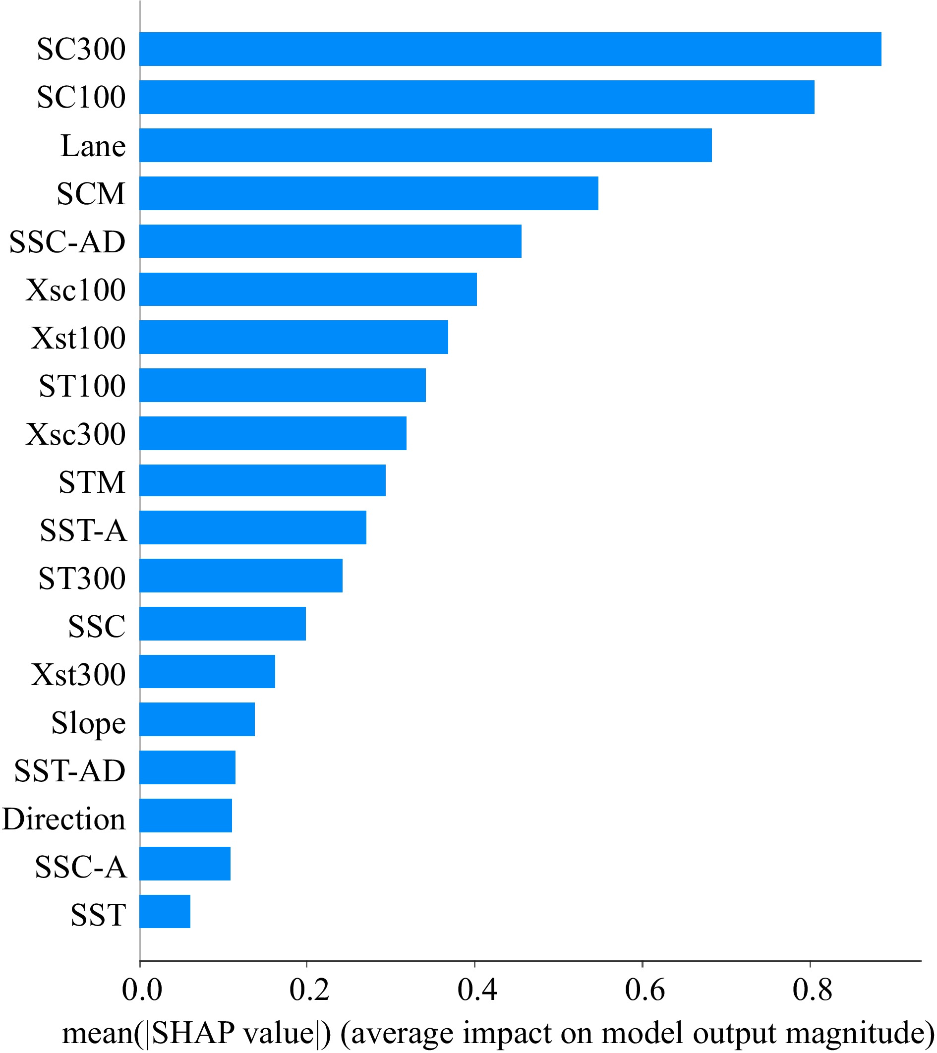
Figure 11.
Feature important score contribution ranking.
-
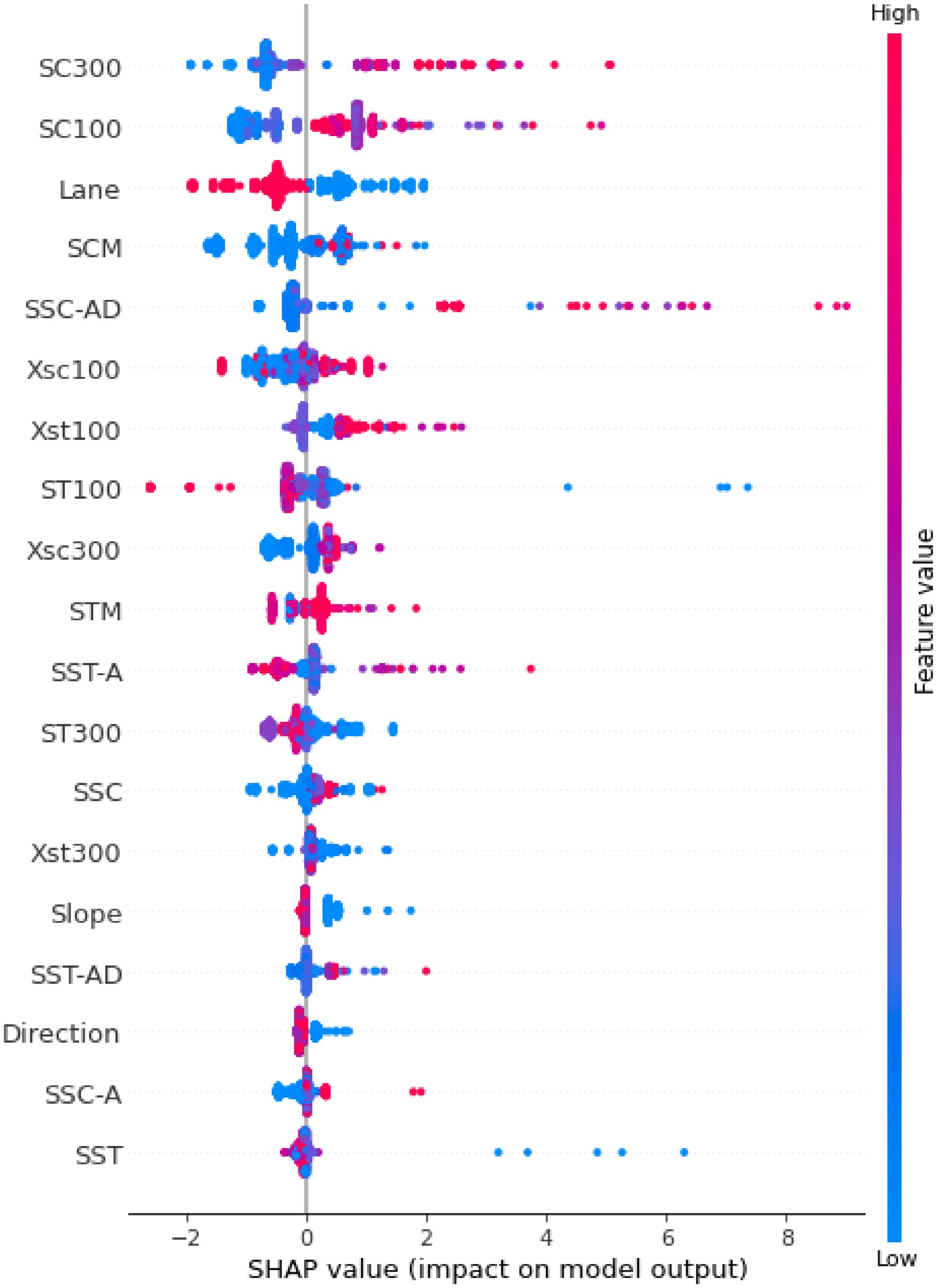
Figure 12.
SHAP value (the positive and negative influence of each variable under the value frame).
-
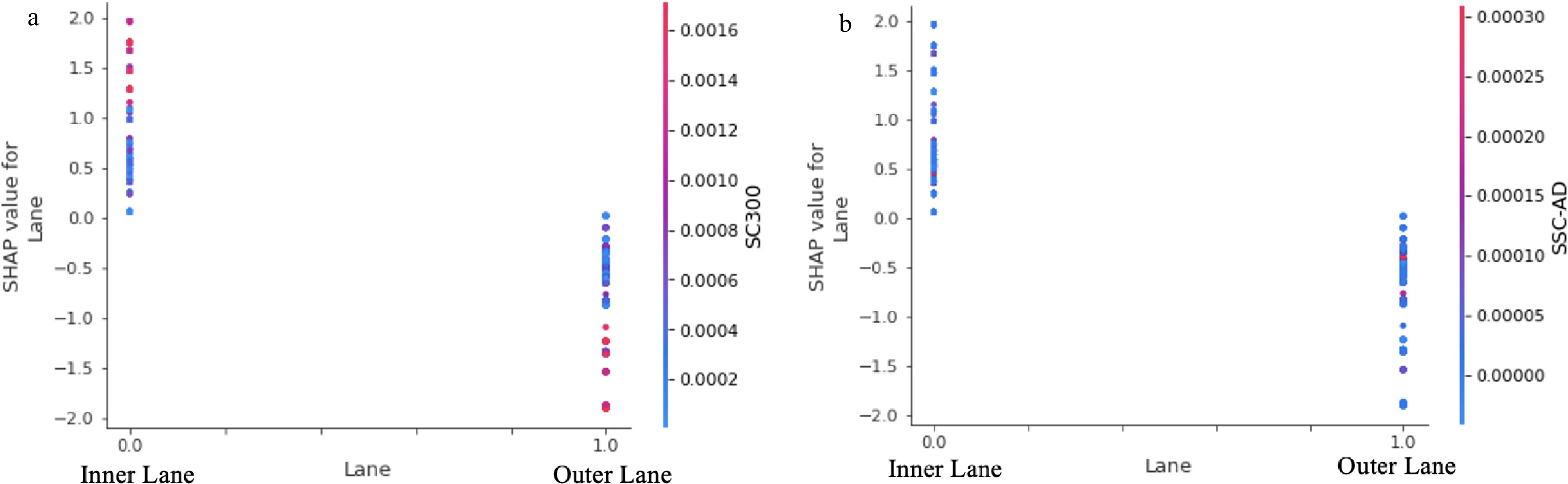
Figure 13.
Lane variable SHAP value mapping.
-
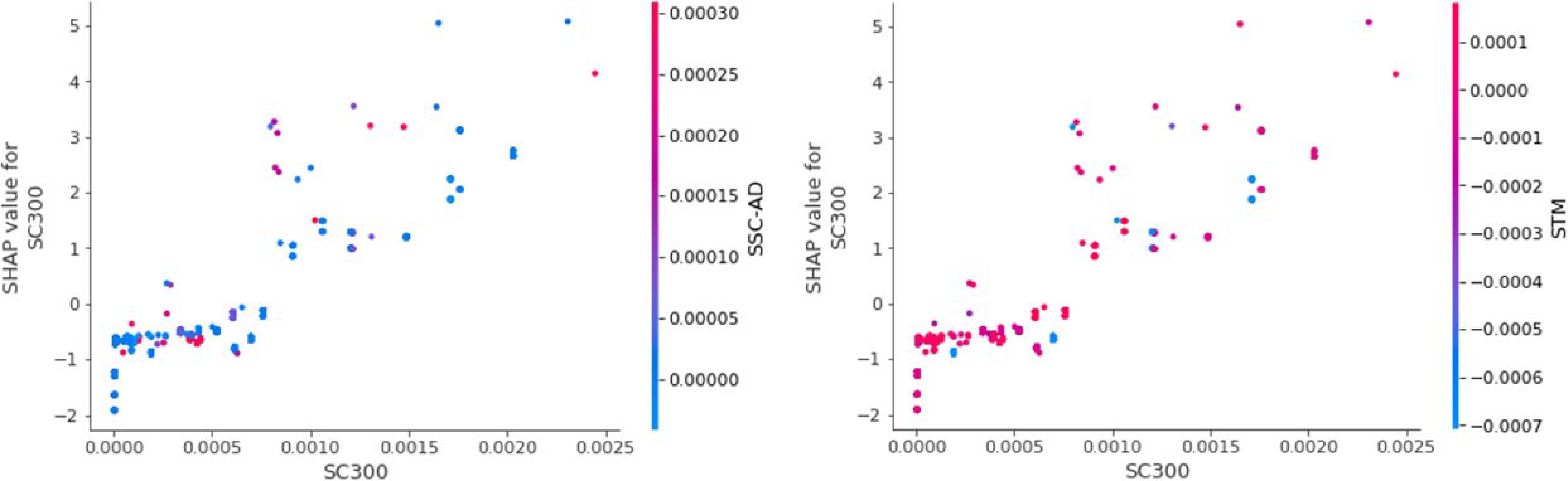
Figure 14.
SHAP value mapping value when SC300 is a single variable (SC300 is m−1).
-
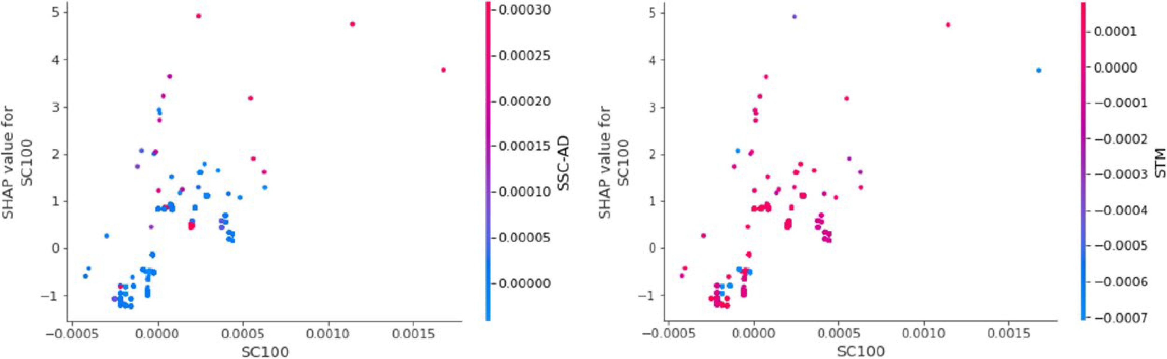
Figure 15.
The mapping relationship between SHAP value when SC100 is a single variable (SC100 is m−1).
-
Block Description Simulation information Containing all the simulation data ACTOR The vehicle used on the simulation senario SELF Containing data of all the object Trajectory (TRACK) Containing all trajectories that the actor does in the simulation scenario Camera Views of the scenario TIS Technology Independent Sensor PreScan sensor simulation Once the simulation starts, the actuator blocks and sensors blocks are initialized directly or indirectly from the data models that come with the experiment Lane Marker sensor Provides information about the lane lines present on the road. Table 1.
Description of the components involved in the simulation scenario.
-
Intersection
PointAVs speed
Range (km/h)Radius
(m)Transition curve
length (m)Slopes
rank (%)JD1
40−100800 105 2−1.5 JD2 800 105 0.5−2.85 JD3 310 160 3−2.5 JD4 310 160 0−2.26 JD5 375 145 2.32−4 JD6 1,100 0 1.2−2.01 JD7 5,900 0 −0.8 − −4 JD8 600 115 −2 Table 2.
Experiment road geometric design parameters.
-
Horizontal alignment Vertical alignment Space combination alignment Code
nameTangent Slope Tangent + slope TT Vertical curve Tangent + vertical curve TV Horizontal curve Slope Horizontal curve + slope CT Vertical curve Horizontal curve + vertical curve CV Spiral curve Slope Spiral curve + slope ST Vertical curve Spiral curve + vertical curve SV Table 3.
Experiment road segment division.
-
Road segment Curvature k calculation formula Torsion $ \tau $ TT 0 0 TV $ \begin{array}{c}\dfrac{1}{{R}_{v}{\left(1+{\left(\dfrac{\left(l+{l}_{b}\right)}{{R}_{v}}+{i}_{1}\right)}^{2}\right)}^{\frac{3}{2}}}\\ \dfrac{\left({l}_{s}+{l}_{a}\right)}{{A}^{2}\left(1+{i}_{1}^{2}\right)}\end{array} $ 0 ST $ \dfrac{\left({l}_{s}+{l}_{a}\right)}{{A}^{2}\left(1+{i}_{1}^{2}\right)} $ $ \dfrac{{i}_{1}\left({l}_{s}+{l}_{a}\right)}{{A}^{2}\left(1+{i}_{1}^{2}\right)} $ SV $ \dfrac{{\left(\dfrac{1}{{R}_{v}^{2}}+{\left(\dfrac{\left({l}_{s}+{l}_{a}\right)}{{A}^{2}}\right)}^{2}\left({\left(\dfrac{\left(l+{l}_{b}\right)}{{R}_{v}}+{i}_{1}\right)}^{2}+1\right)\right)}^{\frac{1}{2}}}{{\left(1+{\left(\dfrac{\left(l+{l}_{b}\right)}{{R}_{v}}+{i}_{1}\right)}^{2}\right)}^{\frac{3}{2}}} $ $ \dfrac{{\left(\dfrac{\left({l}_{s}+{l}_{a}\right)}{{A}^{2}}\right)}^{3}\left(\dfrac{\left(l+{l}_{b}\right)}{{R}_{v}}+{i}_{1}\right)-\dfrac{1}{{A}^{2}{R}_{v}}}{\dfrac{1}{{R}_{v}^{2}}+{\left(\dfrac{\left({l}_{s}+{l}_{a}\right)}{{A}^{2}}\right)}^{2}\left({\left(\dfrac{\left(l+{l}_{b}\right)}{{R}_{v}}+{i}_{1}\right)}^{2}+1\right)} $ CT $ \dfrac{1}{{R}_{h}\left(1+{i}_{1}^{2}\right)} $ $ \dfrac{{i}_{1}}{{R}_{h}\left(1+{i}_{1}^{2}\right)} $ CV $ \dfrac{{\left(\dfrac{1}{{R}_{v}{}^{2}}+\dfrac{1}{{R}_{h}{}^{2}}\left({\left(\dfrac{\left(l+{l}_{b}\right)}{{R}_{v}}+{i}_{1}\right)}^{2}+1\right)\right)}^{\frac{1}{2}}}{{\left(1+{\left(\dfrac{\left(l+{l}_{b}\right)}{{R}_{v}}+{i}_{1}\right)}^{2}\right)}^{\frac{3}{2}}} $ $ \dfrac{\left(\dfrac{\left(l+{l}_{b}\right)}{{R}_{v}}+{i}_{1}\right)\dfrac{1}{{R}_{h}{}^{3}}}{\dfrac{1}{{R}_{v}^{2}}+\dfrac{1}{{R}_{h}^{2}}\left({\left(\dfrac{\left(l+{l}_{b}\right)}{{R}_{v}}+{i}_{1}\right)}^{2}+1\right)} $ Table 4.
Curvature and torsion calculation formula.
-
No. Parameters (independent variables) Symbol definition 1 Lane L 2 Slope S 3 Direction (left turn, right turn) D 4 Upstream 300 m average spatial curvature SC300 5 Upstream 300 m spatial curvature composite index Xsc300 6 Upstream 300 m average spatial torsion ST300 7 Upstream 300 m spatial torsion composite index Xst300 8 Upstream 100 m average spatial curvature SC100 9 Upstream 100 m spatial curvature composite index Xsc300 10 Upstream 100 m average spatial torsion ST100 11 Upstream 100 m spatial torsion composite index Xst100 12 Maximum sudden change in spatial curvature nearest to the road section SCM 13 Maximum sudden change in spatial torsion nearest to the road section STM 14 Spatial curvature in the section SCS 15 Curvature difference of adjacent road section SCS-AD 16 Average curvature difference of adjacent road section SCS-A 17 Spatial curvature torsion SCT 18 Torsion difference of adjacent road section STS-AD 19 Average torsion difference of adjacent road section STS-A Table 5.
Space alignment parameters index.
-
Spatial parameters Autonomous vehicle Conventional vehicle Upstream 300 m average spatial curvature (SC300) 10% of the impact.
When SC300 is higher, it has a positive impact on TD.
When the AV is driving on the downhill road section, the TD is not affected.17% of the impact factors.
When SC300 is higher, the TD is significantly affected, and the larger SC300 is the more restrained the TD on the downhill section
Upstream 100 m average spatial curvature (SC100)8% of the impact factors.
Has a positive and negative impact on the TD.
Increasing his value does not have a significant impact on the TD due to the AV's rapid reaction time.10.9% of the impact factors
The values remain between positive and negative.
SC100 has no direct impact on the deviation of the driving trajectory. Due to the lack of time for the driver to adjust the vehicle during the upstream 100, the deviation value of the driving trajectory when the vehicle is in the corresponding section remains the sameLane 7% of the impact factors.
The AV's TD is positively affected when it is driving in the inner lane and negatively affected when it is driving in the outer lane.
When AV is making a left turn, it tends to shift outward.12.2% of the impact factors.
When considering the interaction with SC300, the larger the SC300 in the left-turn section, the more restrained the deviation of the driving trajectory.
A serious left deviation occurs When a conventional vehicle is making a left turn.Table 6.
AVs and conventional TD behavior comparaison.
Figures
(15)
Tables
(6)