-
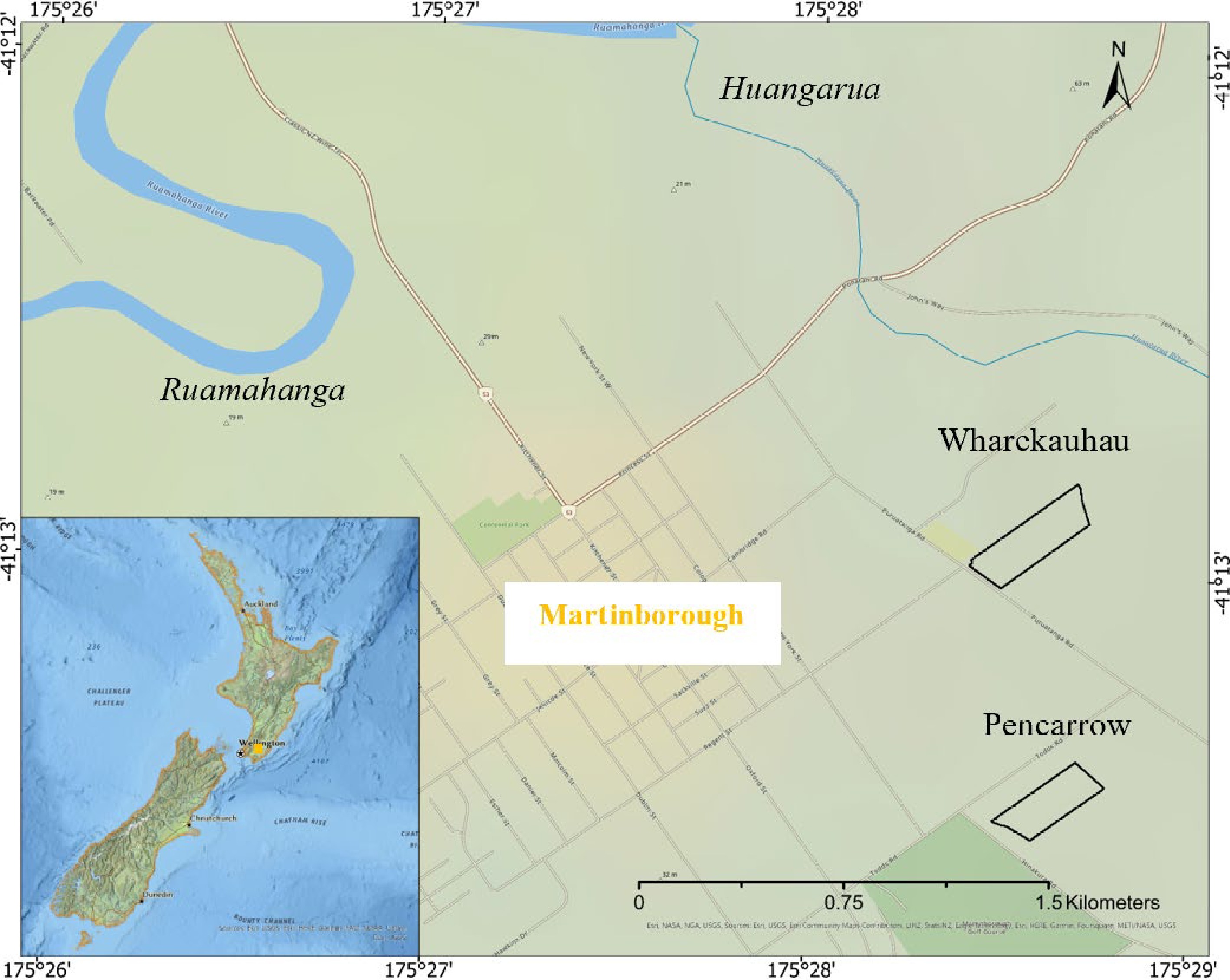
Figure 1.
Location of study vineyards (Source: Esri, USGS).
-
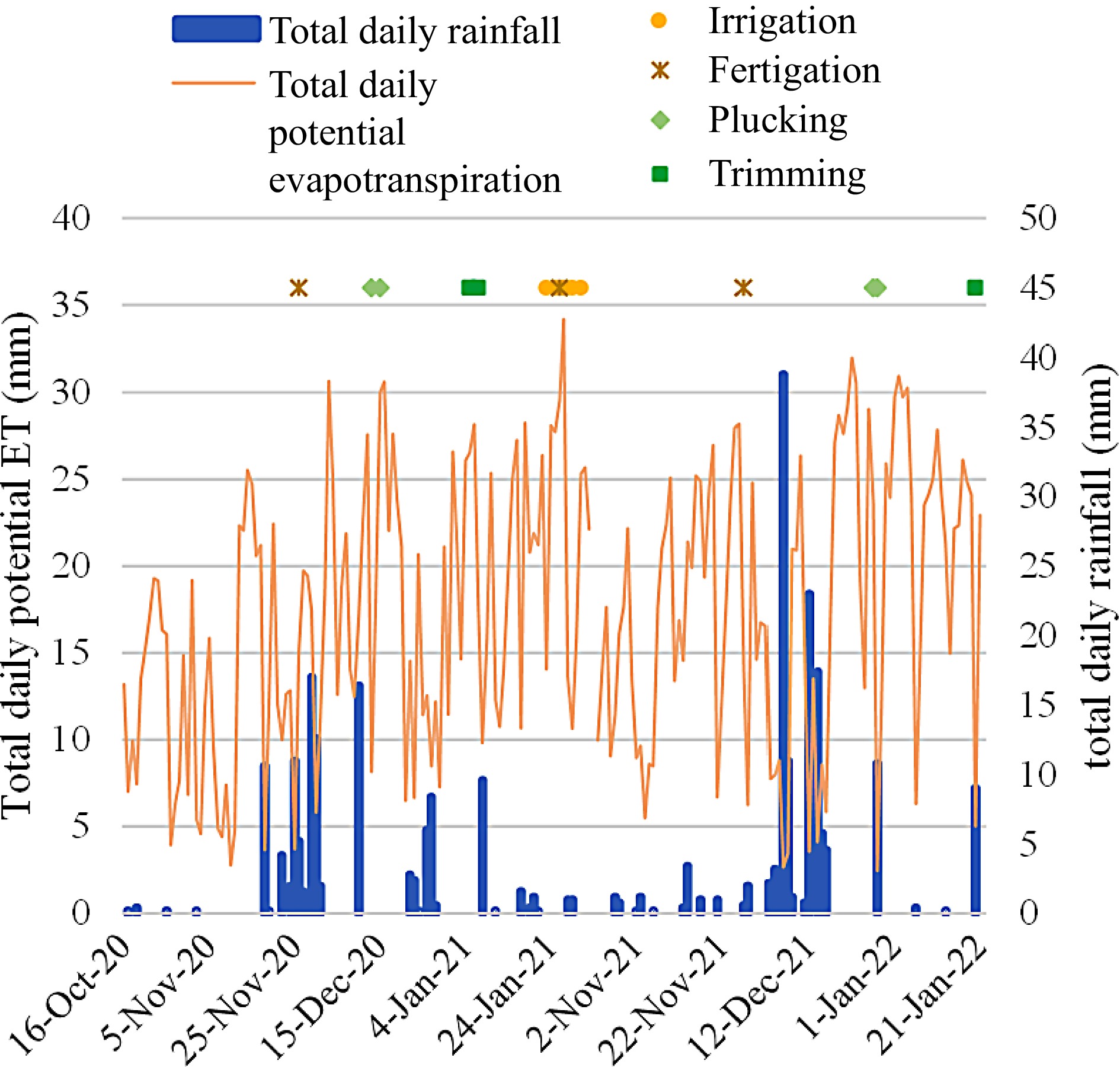
Figure 2.
Total daily potential evapotranspiration and total daily rainfall provided by an on-site weather station, with cultivation practices implemented during the two growing seasons.
-
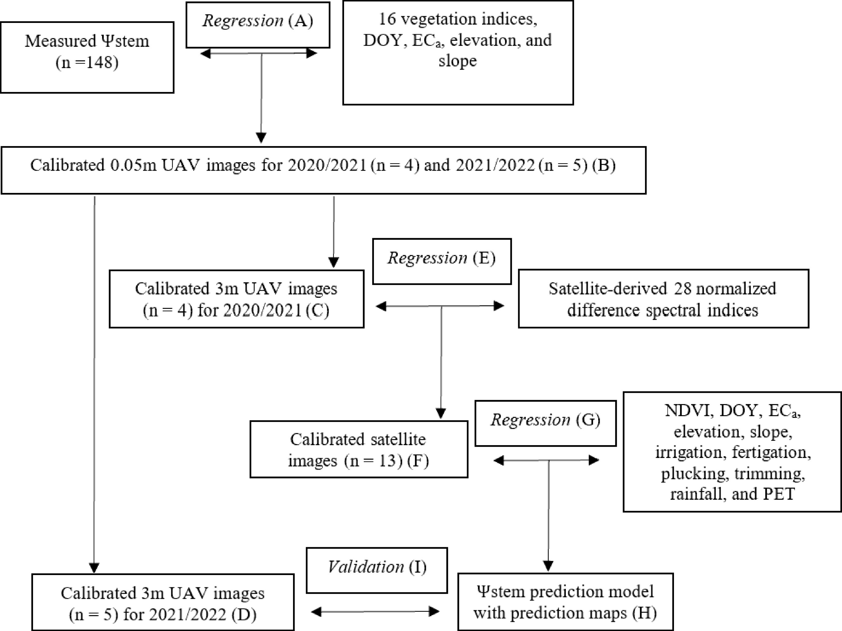
Figure 3.
Overview of the workflow. UAV = uncrewed aerial vehicle; DOY = day of the year; NDVI = normalized difference vegetation index; ECa = apparent electrical conductivity; PET = potential evapotranspiration.
-
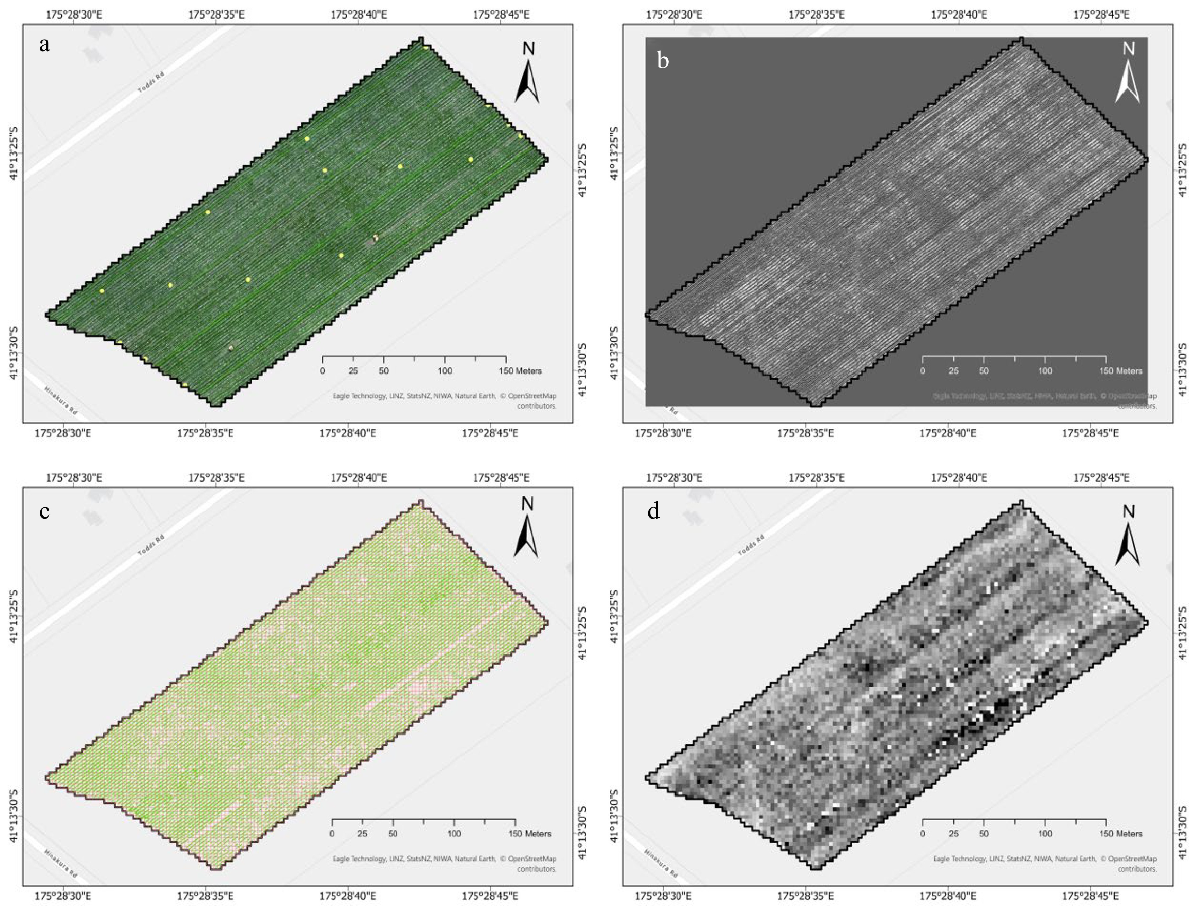
Figure 4.
An illustration of generating a downscaled 3 m UAV image for each UAV survey date. (a) UAV image is presented as RGB composites, with measured Ѱstem presented as yellow points. (b) Calibrated 0.05 m UAV image exhibiting Ѱstem estimation. (c) Green pixels are pure pixels representing grapevines after clipping pixels of interrow, overlaid with 3 m red grids. (d) Downscaled 3 m UAV image after spatial aggregation of pixels in red grids.
-
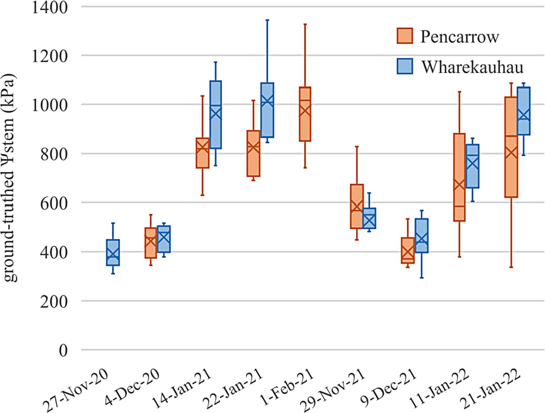
Figure 5.
Box plot of measured Ψstem collected during two growing seasons at Pencarrow (n = 86) and Wharekauhau (n = 62) vineyards. X symbols refer to the average values on the survey dates. Horizontal lines in the boxes refer to median values on the survey dates.
-
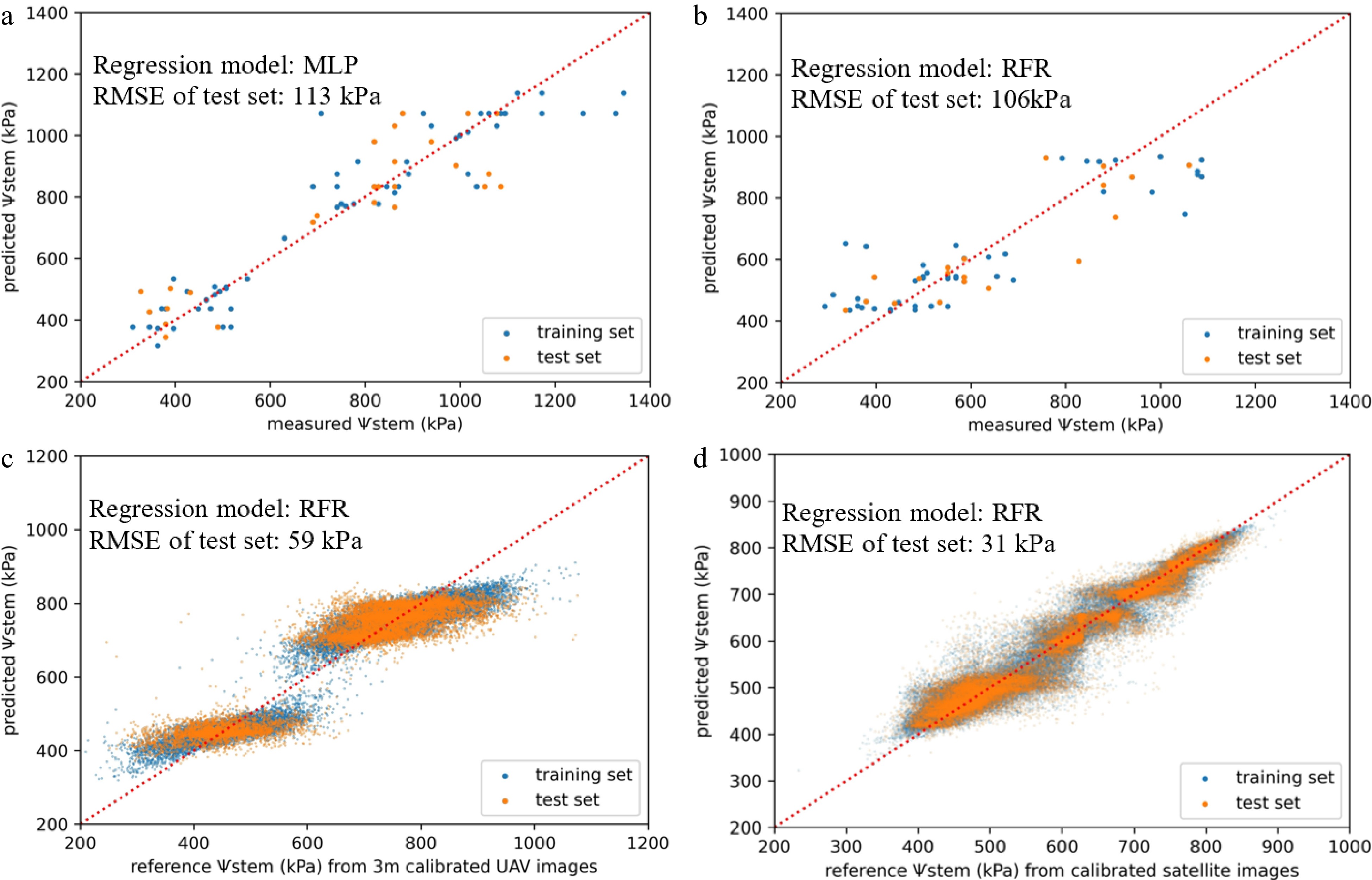
Figure 6.
Scatter plots between predicted Ѱstem and measured or reference Ѱstem (kPa) for the training and test sets of (a) the calibration of UAV images acquired in 2020/2021. (b) Calibration of UAV images acquired in 2021/2022. (c) Calibration of satellite (PS) images. (d) Prediction of Ѱstem in 2020/2021. Red dashed lines are 1:1 lines. Samples from the two study vineyards are considered collectively in each regression model.
-
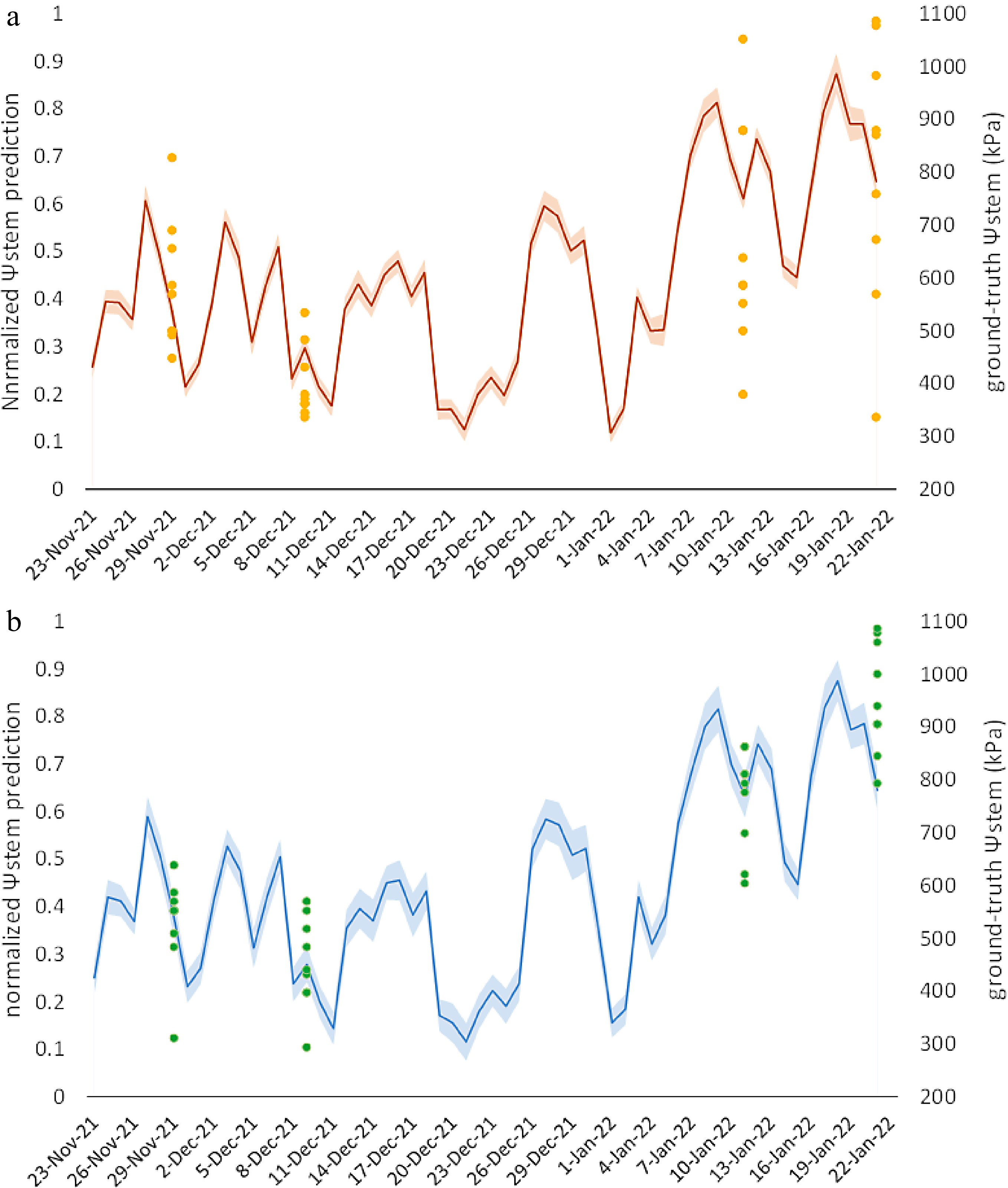
Figure 7.
The temporal patterns of normalized Ψstem prediction (lines) during the growing season in 2021/2022, with the measured Ψstem measurements (points) for (a) Pencarrow and (b) Wharekauhau. The shaded bands bordering the lines encompass one standard deviation.
-
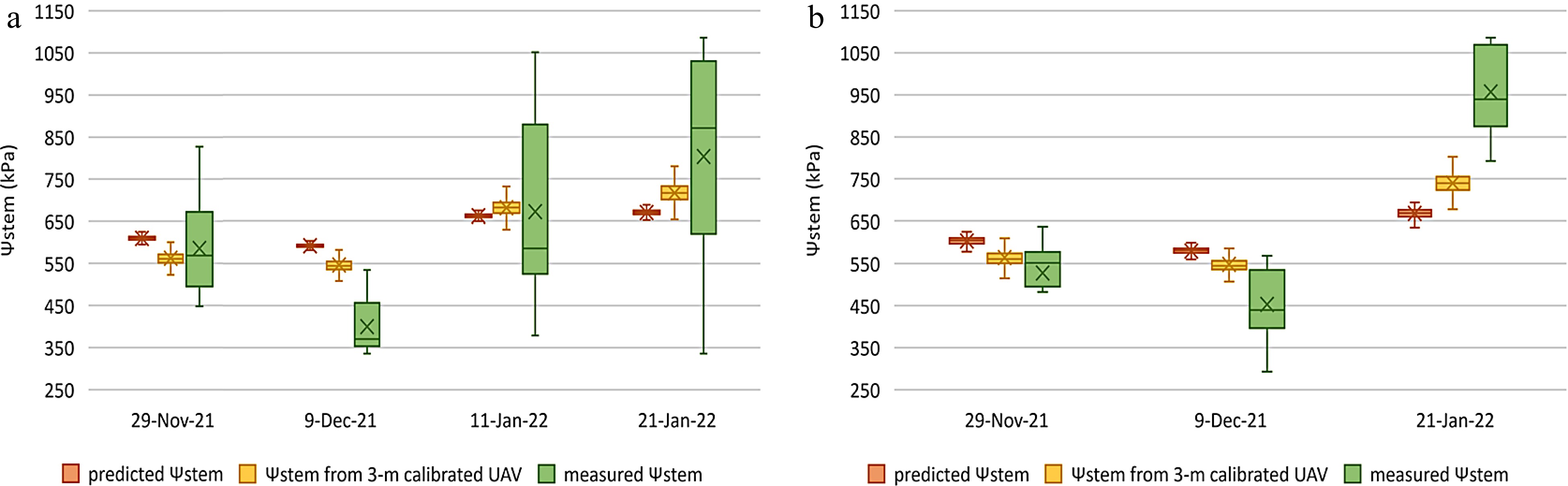
Figure 8.
Box plots of predicted Ψstem values, Ψstem values acquired from 3 m calibrated UAV images, and measured Ψstem values for each survey date at the (a) Pencarrow and (b) Wharekauhau vineyards. UAV = uncrewed aerial vehicle, and Ψstem = stem water potential.
-
Acquisition date Data source Time gap (d) 15/11/2020 Satellite − 16/11/2020 Satellite − 27/11/2020 Measured/UAV − 02/12/2020 Satellite − 04/12/2020 Measured/UAV 1 05/12/2020 Satellite 15/12/2020 Satellite − 17/12/2020 Satellite − 31/12/2020 Satellite − 04/01/2021 Satellite − 14/01/2021 Measured/UAV/
Satellite0 15/01/2021 Satellite − 22/01/2021 Measured/UAV 1 23/01/2021 Satellite 26/01/2021 Satellite − 01/02/2021 Measured/UAV 1 02/02/2021 Satellite 23/11/2021 UAV − 29/11/2021 Measured/UAV − 09/12/2021 Measured/UAV − 11/01/2022 Measured/UAV − 21/01/2022 Measured/UAV − Table 1.
Details of data acquisition for measured Ψstem, DJI Phantom 4 multispectral UAV imagery, and PlanetScope satellite imagery. The orange letterings indicate the UAV-satellite image pairs used in the second calibration. UAV = uncrewed aerial vehicle.
-
Vegetation index Formula Reference Red Edge Chlorophyll Index (NIR/Red edge) − 1 [39] Difference Vegetation Index NIR − Red [40] Enhanced Vegetation Index 2.5 × (NIR − Red)/(NIR + 6 * Red − 7.5 × Blue + 1) [41] Excess Green Index 2 × Green − Red − Blue [42] Green Normalized Difference
Vegetation Index(NIR − Green)/(NIR + Green) [43] Modified Chlorophyll Absorption Ratio Index ((Red edge − Red) − 0.2 × (Red edge − Green)) ×
(Red edge/Red)[44] Modified Soil Adjusted
Vegetation Index(2 × NIR+1 − ((2 × NIR + 1)2 − 8 × (NIR − Red))1/2)/2 [45] Modified Triangular
Vegetation Index1.2 × (1.2 × (NIR − Green) − 2.5 × (Red − Green)) [46] Normalized Difference
Red Edge Index(NIR − Red edge)/(NIR + Red edge) [47] Normalized Difference
Vegetation Index(NIR − Red)/(NIR + Red) [48] Normalized Difference
Green/Red Index(Green − Red)/(Green + Red) [40] Optimized Soil Adjusted
Vegetation Index(NIR − RED)/(NIR + Red + 0.16) [49] Red: Green Ratio Red/Green [50] Simple Ratio NIR/Red [51] Transformed Chlorophyll
Absorption Reflectance Index3 × ((Red edge − Red) − 0.2 × (Red edge − Green) ×
(Red edge/Red))[52] Visible Atmospherically
Resistant Index(Green − Red)/(Green + Red − Blue) [53] Table 2.
List of vegetation indices used in this study.
-
Predictor Note Number DOY The number is added on along the growing
season.1 NDVI Collected in late November for the 2020/2021 and 2021/2022 seasons separately. 1 ECa − 1 Elevation − 1 Slope − 1 Total daily rainfall The rainfall amounts on each day of the 30-day
period beforehand was used as a predictor.30 Total daily PET The PET amounts on each day of the 30-day
period beforehand was used as a predictor.30 Irrigation and
FertigationThe water input amounts, either sourced from
irrigation or fertigation, on each day of the 30-day period beforehand was used as a predictor.30 Plucking and Trimming The occurrence of the events on each day of the 30-day period beforehand was used as a
predictor.30 Table 3.
A summary for the predictors used in developing the Ѱstem prediction model. DOY = day of the year; NDVI = normalized difference vegetation index; ECa = apparent electrical conductivity; PET = potential evapotranspiration.
-
Modeling purpose Regression model Data size of measured
or reference ΨstemRMSE of the
training set (kPa)RMSE of the
test set (kPa)Calibration of UAV images
acquired in 2020/2021
(Fig. 3a)Multilayer
perceptron85 96 113 Calibration of UAV images
acquired in 2021/2022
(Fig. 3a)Random forest
regression63 121 106 Calibration of
Satellite images (Fig. 3e)Random forest
regression42,234 47 59 Prediction of Ψstem (Fig. 3g) Random forest
regression151,580 25 31 Table 4.
Results of modeling performance. UAV = uncrewed aerial vehicle; Ψstem = stem water potential; RMSE = root mean square error.
-
Pencarrow Wharekauhau r 0.89* 0.87* Significance levels are noted as * when p ≤ 0.001. Table 5.
Results of similarity analysis, presented by the Pearson correlation coefficient (r), represent the consistency between predicted and reference Ψstem maps across four survey dates for the two study vineyards.
-
Survey date Vineyard Data source Mean SD CV 29th November 2021 Pencarrow Predicted Ψstem 609 5.59 0.92 Ψstem from 3 m calibrated UAV 562 18.11 3.22 Measured Ψstem 585 113.93 19.47 Wharekauhau Predicted Ψstem 603 9.26 1.53 Ψstem from 3 m calibrated UAV 565 21.86 3.87 Measured Ψstem 528 87.31 16.55 9th December 2021 Pencarrow Predicted Ψstem 593 5.03 0.85 Ψstem from 3 m calibrated UAV 547 15.19 2.78 Measured Ψstem 400 64.25 16.05 Wharekauhau Predicted Ψstem 580 8.95 1.54 Ψstem from 3 m calibrated UAV 548 17.42 3.18 Measured Ψstem 453 82.18 18.14 11th January 2022 Pencarrow Predicted Ψstem 662 4.84 0.73 Ψstem from 3 m calibrated UAV 681 19.53 2.87 Measured Ψstem 672 204.27 30.39 21st January 2021 Pencarrow Predicted Ψstem 670 6.73 1.01 Ψstem from 3 m calibrated UAV 717 22.86 3.19 Measured Ψstem 803 233.27 29.03 Wharekauhau Predicted Ψstem 668 10.35 1.55 Ψstem from 3 m calibrated UAV 740 24.67 3.34 Measured Ψstem 957 99.35 10.39 Table 6.
Summary statistics for predicted Ψstem, Ψstem acquired from 3 m calibrated UAV images, and measured Ψstem for each survey date at the Pencarrow and Wharekauhau vineyards. UAV = uncrewed aerial vehicle; SD = standard deviation; CV = coefficient of variation.
Figures
(8)
Tables
(6)