-
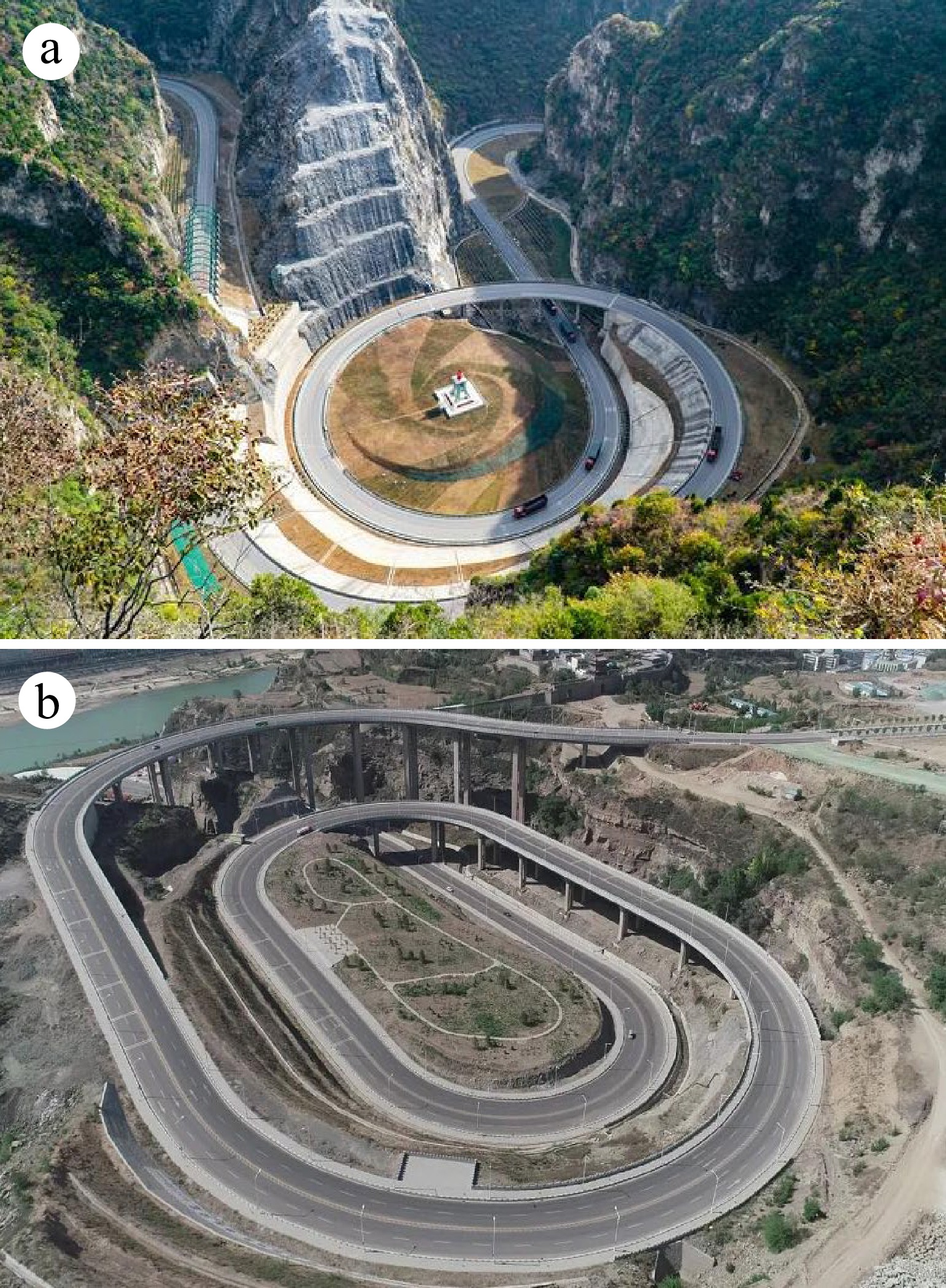
Figure 1.
Common gyroidal roads in China. (a) Longmen ancient road at the junction of Henan and Shanxi; (b) East line mountain road project in Fugu County, Yulin City, Shaanxi Province.
-
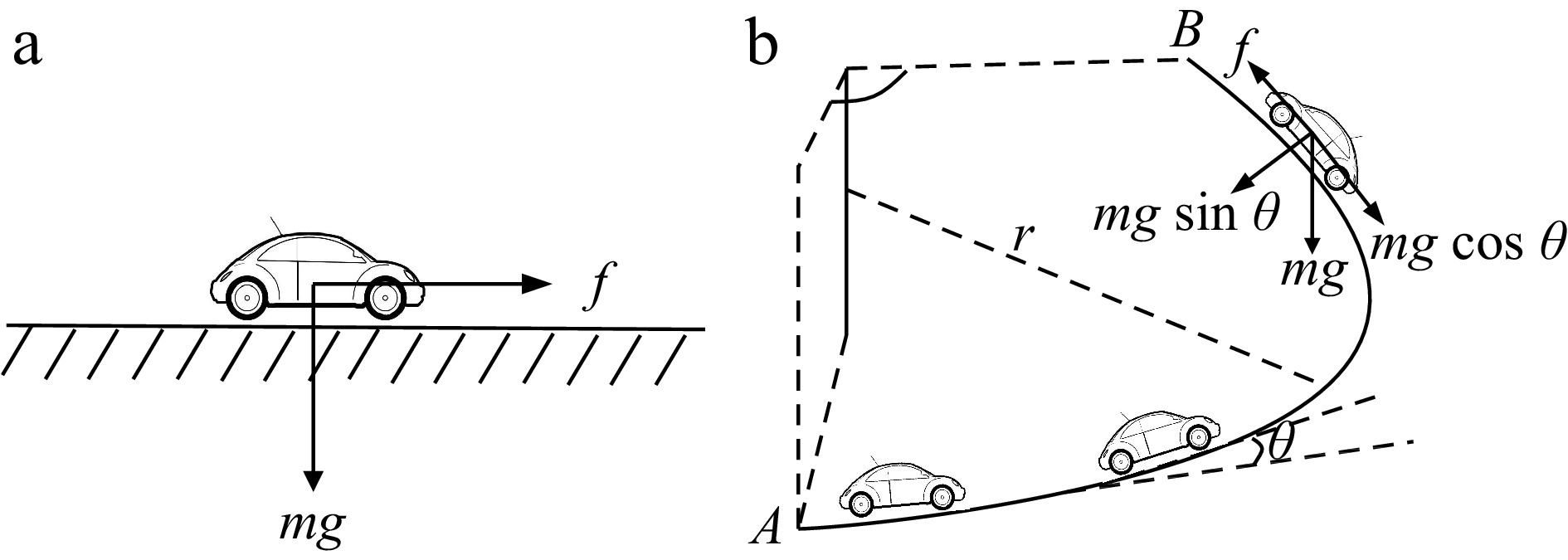
Figure 2.
Illustration of vehicle forces on different road scenes, (a) horizontal or regular road, (b) gyroidal road.
-
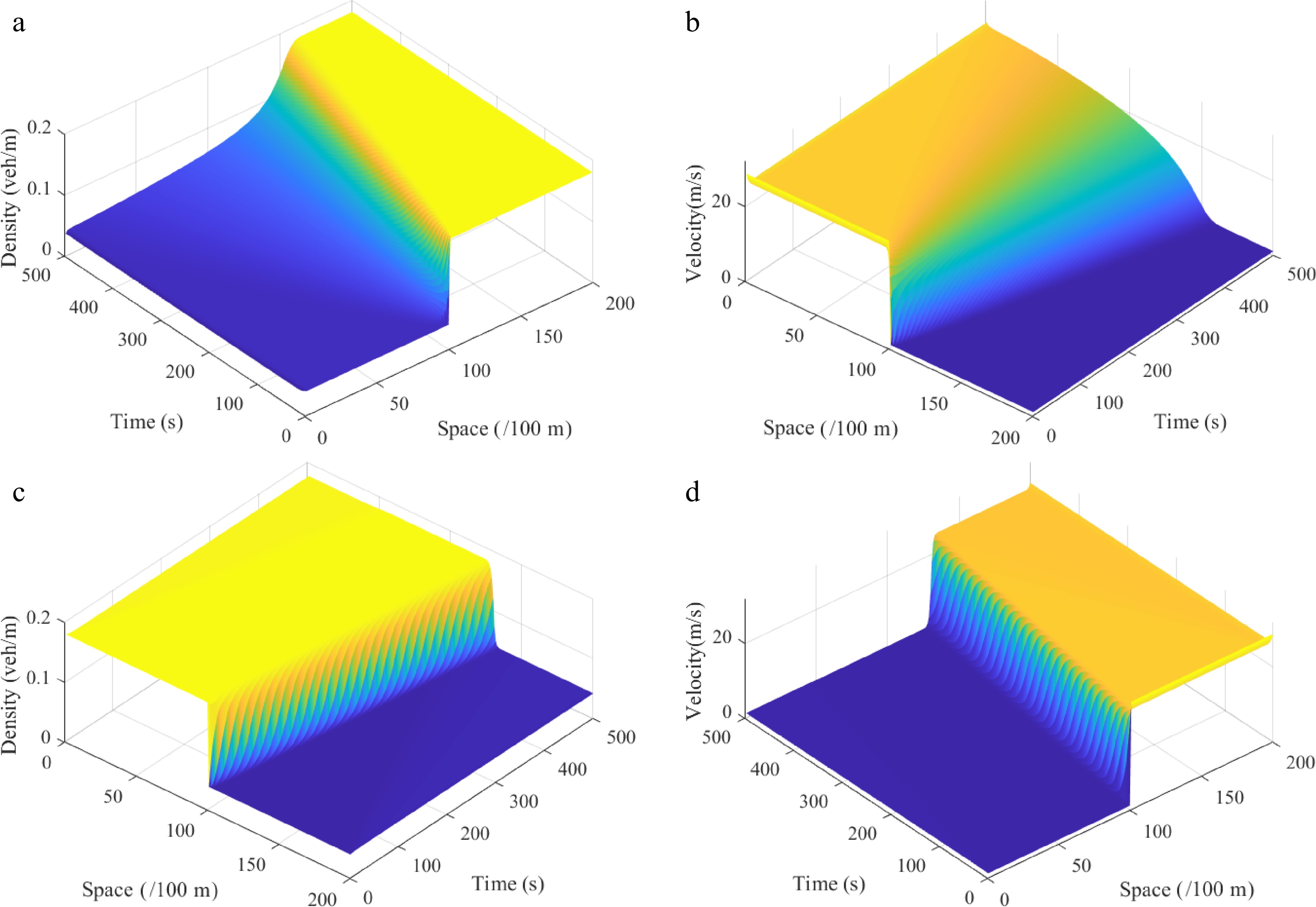
Figure 3.
Shock waves under the Riemann initial condition (i), where: (a) density
$ \rho (\varphi ,t) $ $ \omega r $ $ \rho (\varphi ,t) $ $ \omega r $ $ \theta {\text{ = }} $ -
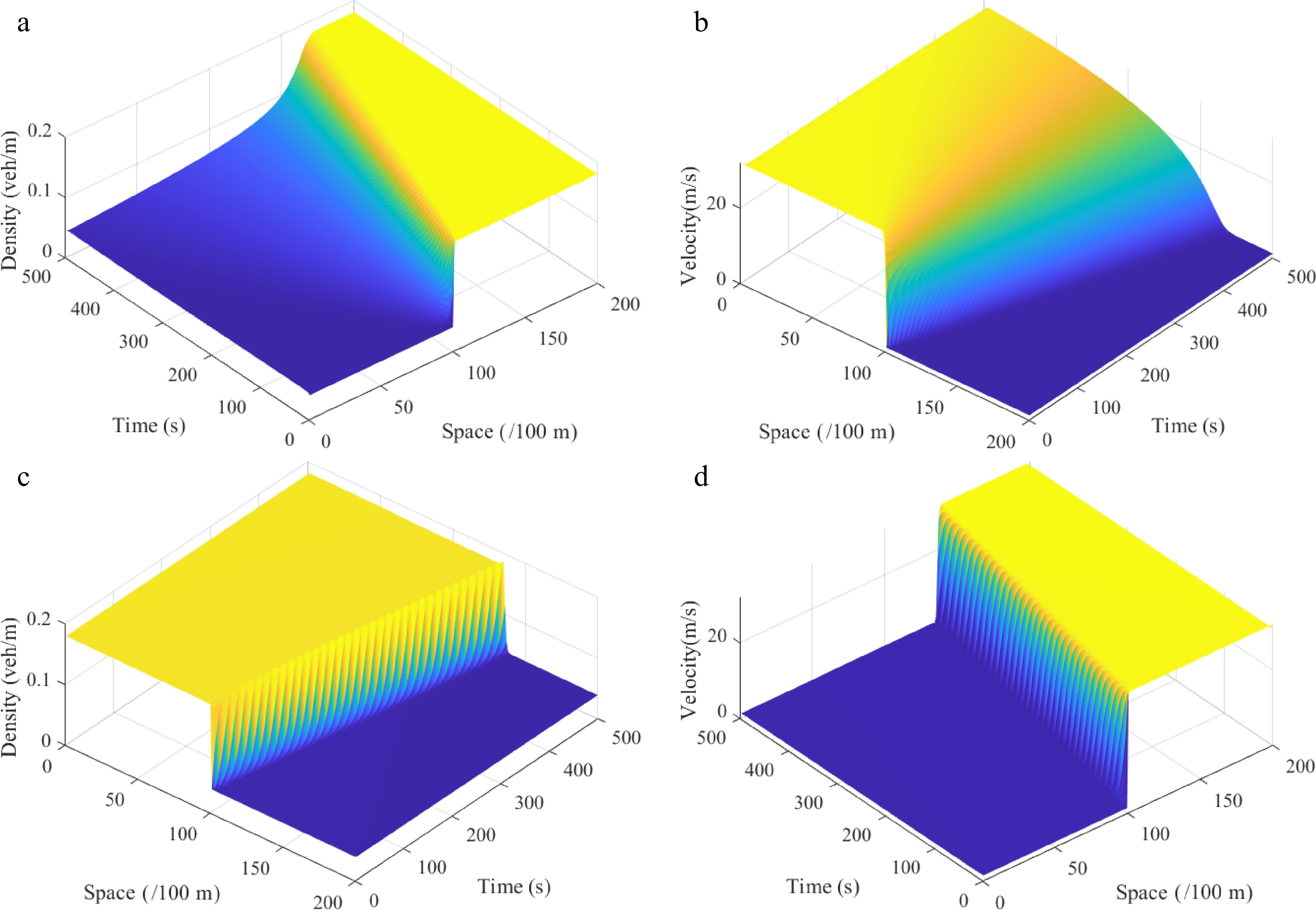
Figure 4.
Shock waves under the Riemann initial condition (i), where: (a) density
$ \rho (\varphi ,t) $ $ \omega r $ $ \rho (\varphi ,t) $ $ \omega r $ $\theta$ -
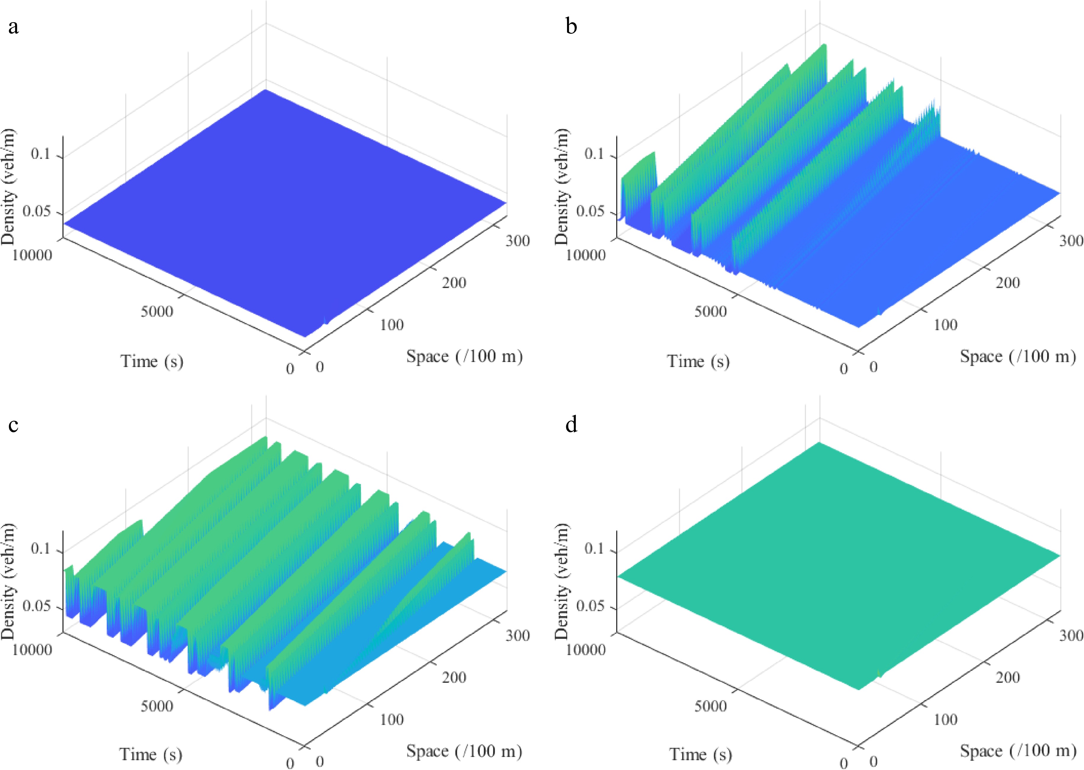
Figure 5.
Spatiotemporal diagram of density waves affected by the initial disturbance under different initial densities ρ0, where: (a) ρ0 = 0.042 veh/m; (b) ρ0 = 0.051 veh/m; (c) ρ0 = 0.065 veh/m; (d) ρ0 = 0.079 veh/m. (l = 2, θ = 0, r = 75).
-
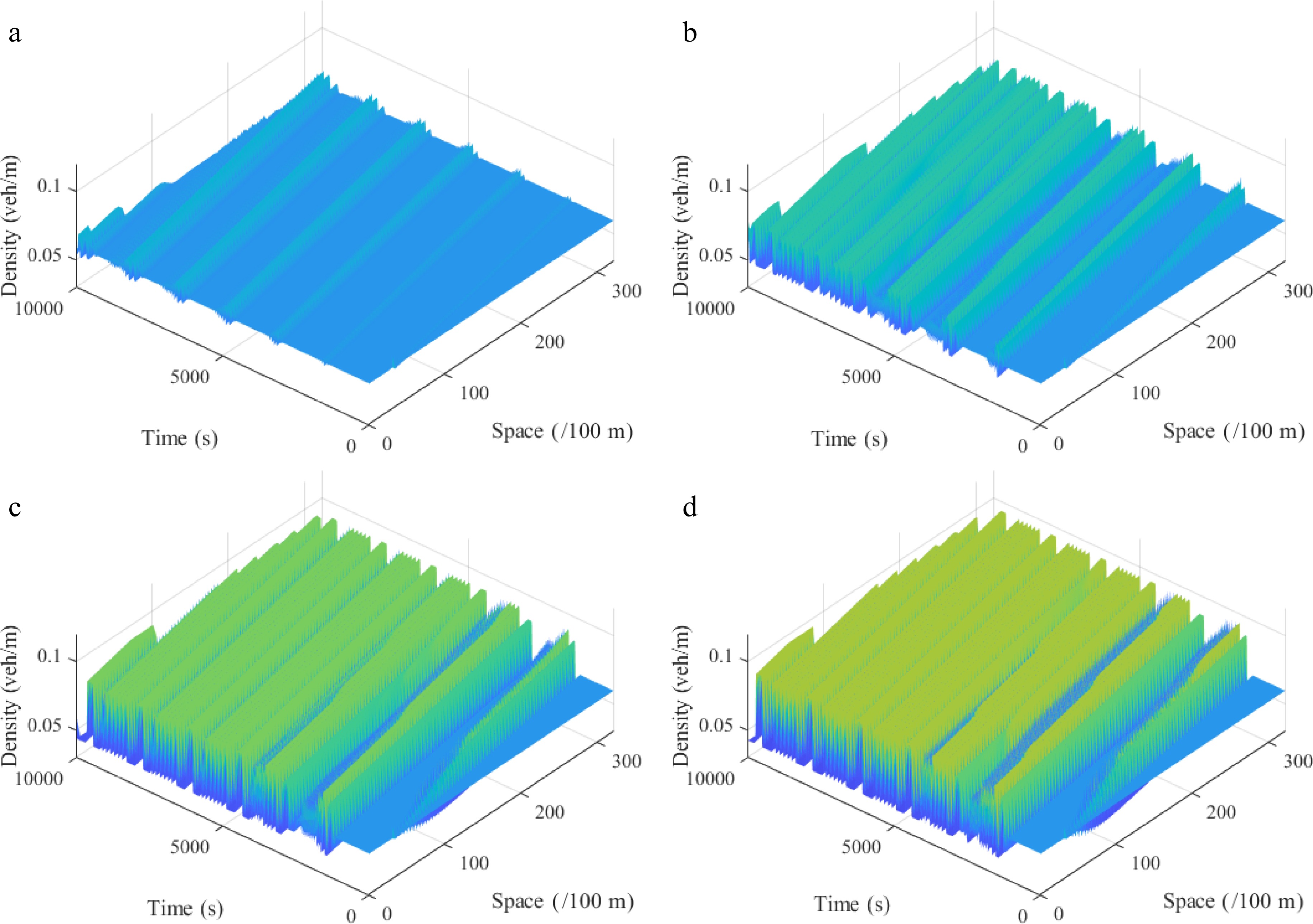
Figure 6.
Spatiotemporal diagram of density waves affected by the initial disturbance under different slope angles θ, where: (a) θ = −10; (b) θ = −5; (c) θ = 5; (d) θ = 10. (l = 2, ρ0 = 0.06, r = 75).
-
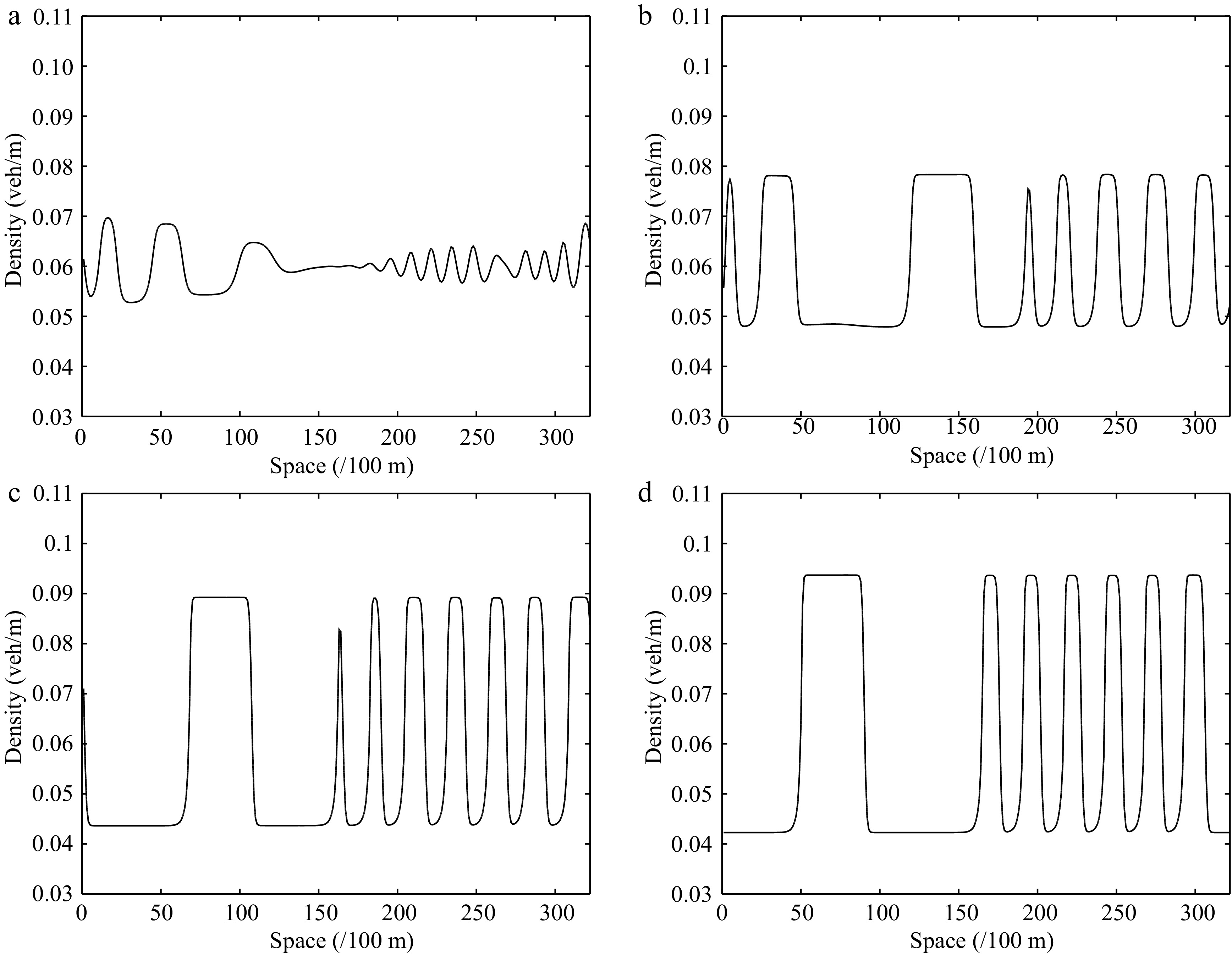
Figure 7.
Instantaneous density distribution of traffic flow corresponding to Fig. 6 at t = 3,000 s.
-
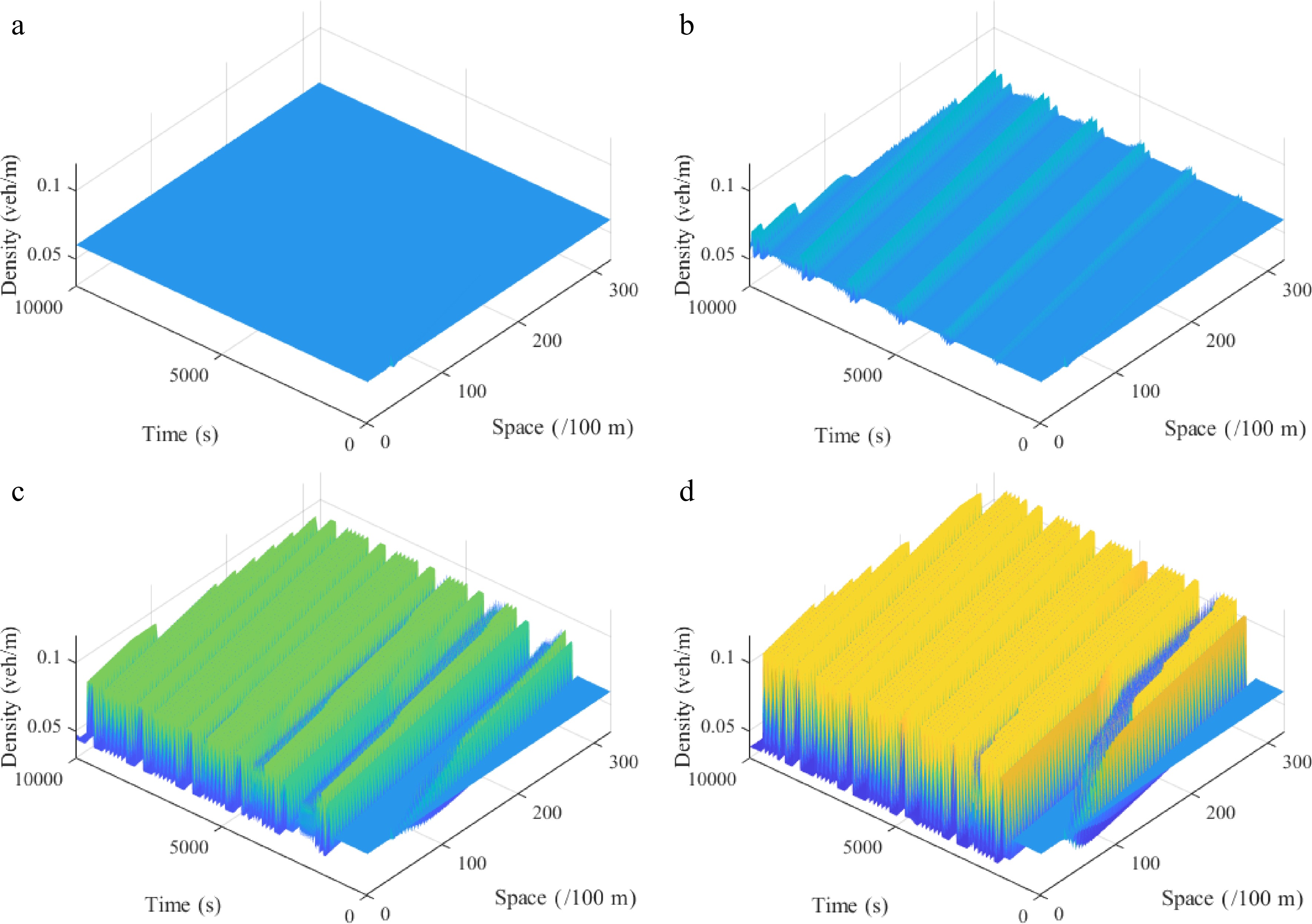
Figure 8.
Spatiotemporal diagram of density waves affected by the initial disturbance corresponding to different curvature radiuses r under the downhill scenario, where: (a) r = 50; (b) r = 70; (c) r = 90; (d) r = 120. (
$ {\rho _0} $ $ \theta $ $ l $ -
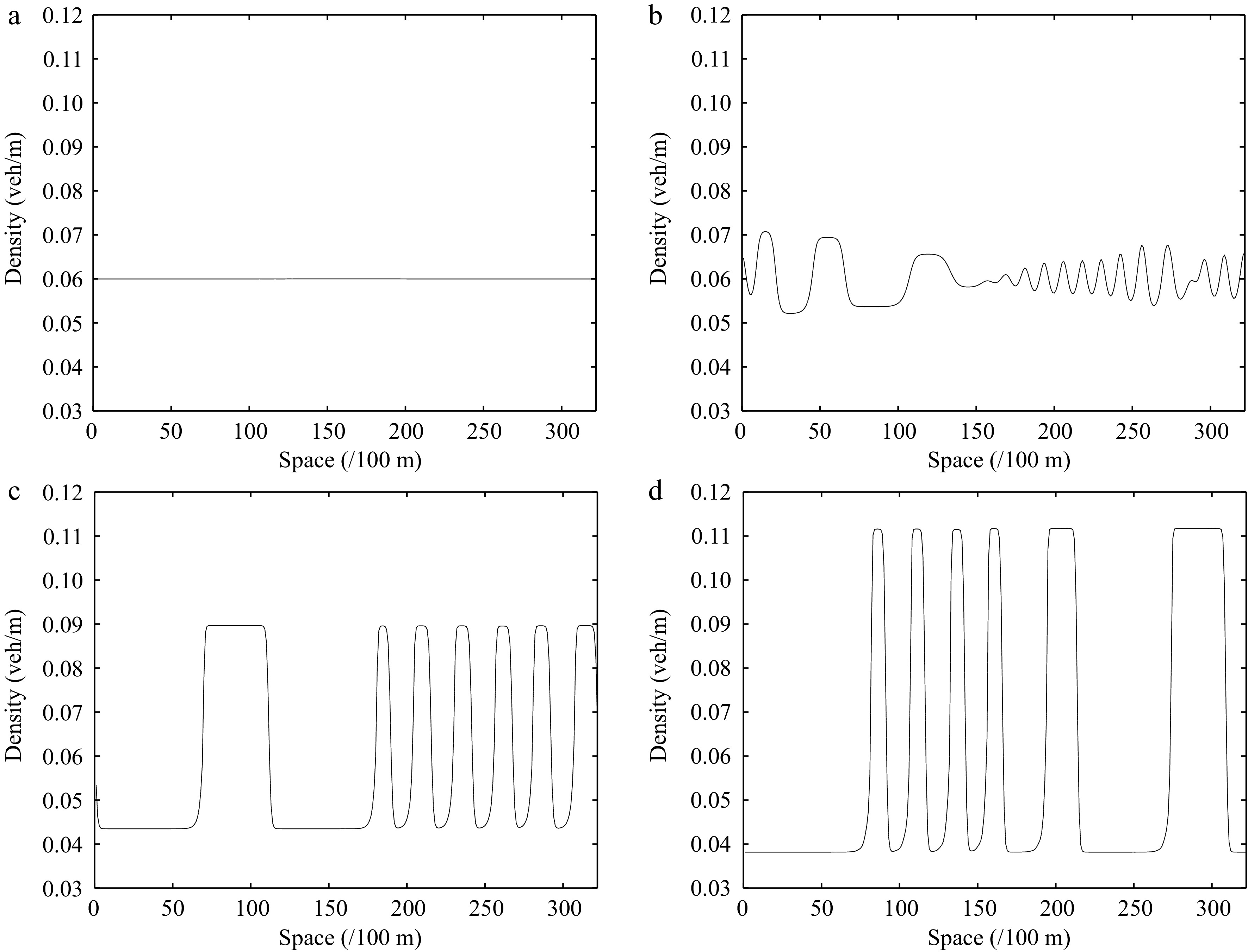
Figure 9.
Instantaneous density distribution of road traffic flow corresponding to Fig. 8 at t = 3,000 s.
-
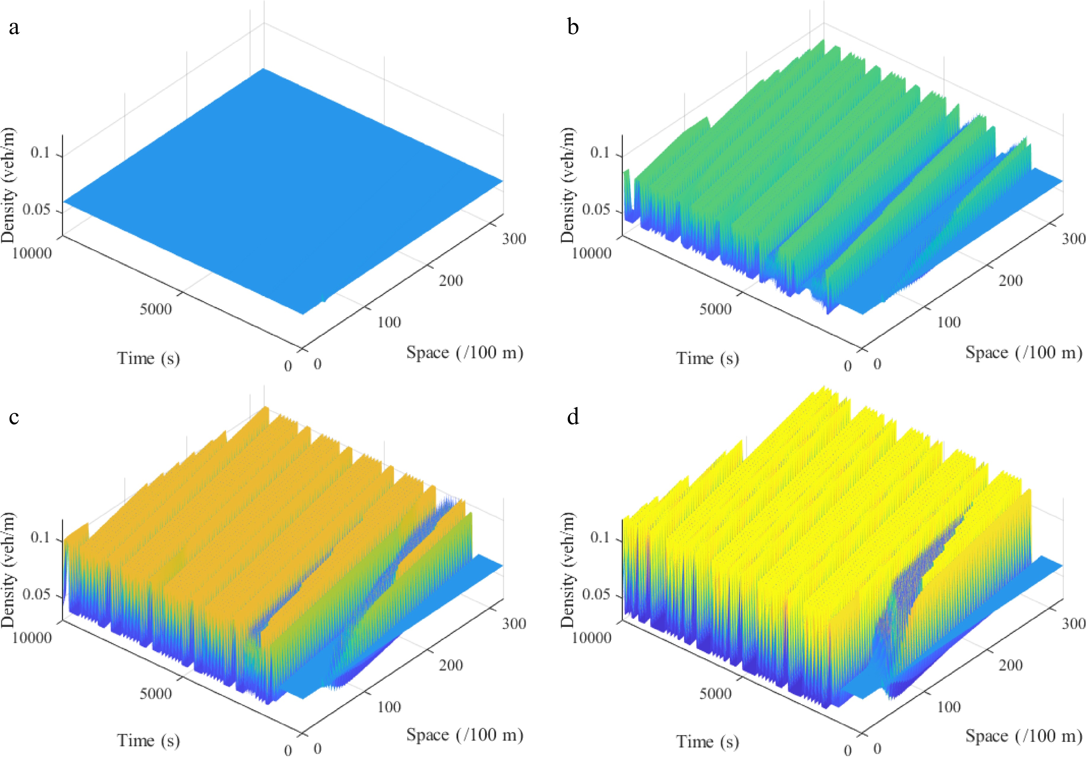
Figure 10.
Spatiotemporal diagram of density waves affected by the initial disturbance corresponding to different curvature radiuses r under the uphill scenario, where: (a) r = 50; (b) r = 70; (c) r = 90; (d) r = 120. (
$ {\rho _0} $ $ \theta $ $ l $ -
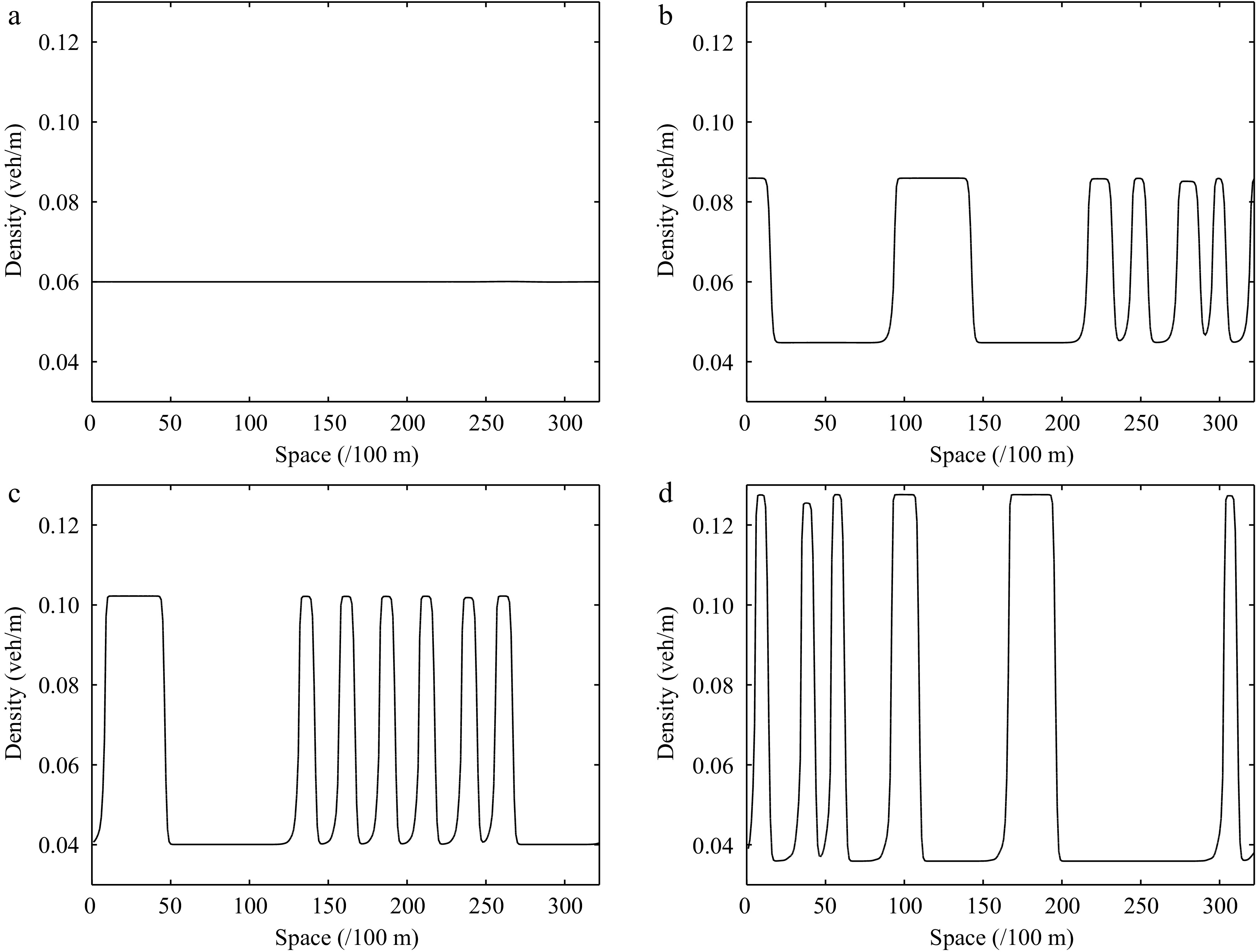
Figure 11.
Instantaneous density distribution of road traffic flow corresponding to Fig. 10 at t = 3,000 s.
-
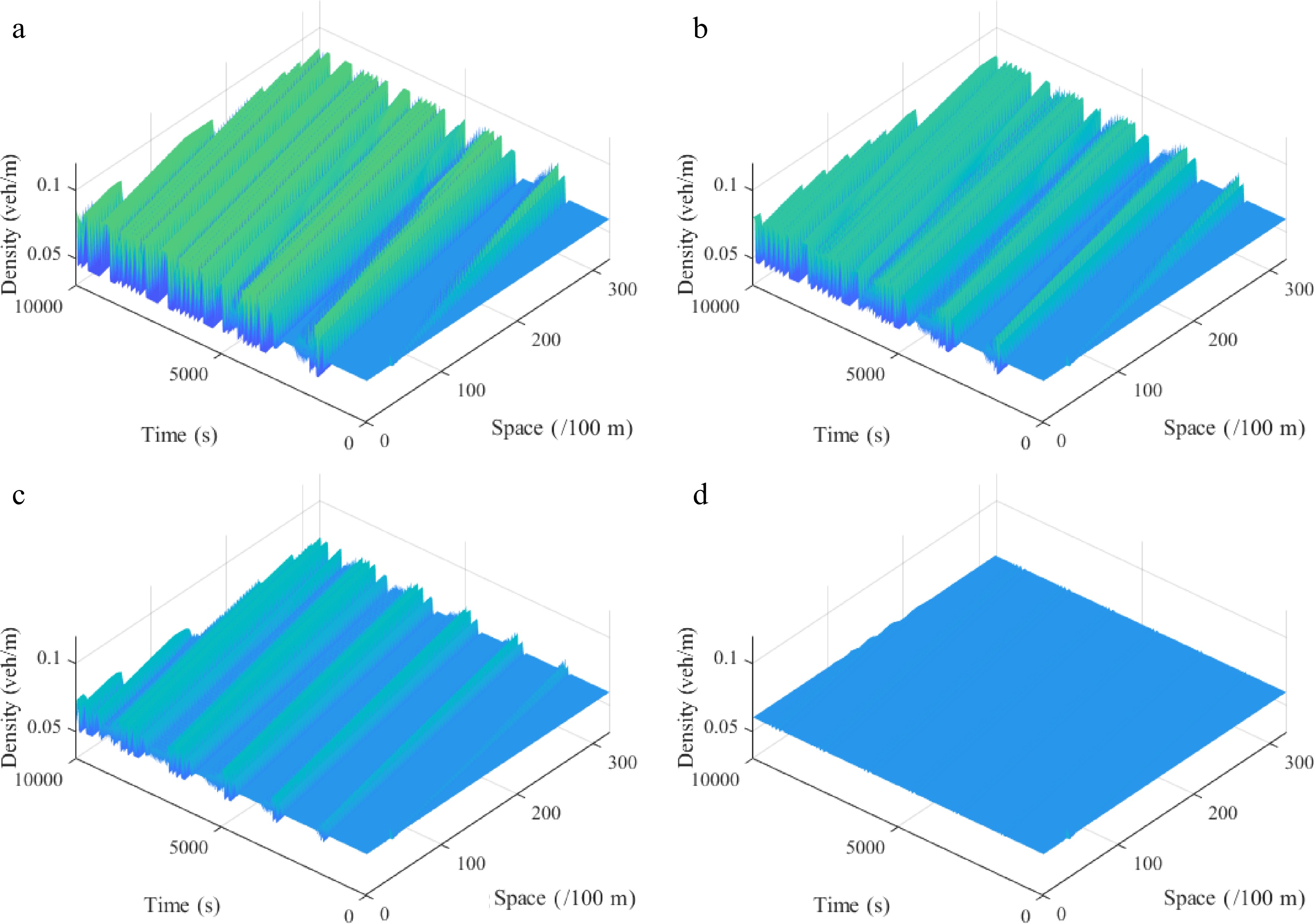
Figure 12.
Spatiotemporal diagram of density waves affected by the initial disturbance corresponding to different values of parameter l under a downhill scenario, where: (a) l = 0; (b) l = 1; (c) l = 2; (d) l = 3. (
$ {\rho _0} $ $ \theta $ $ r $ -
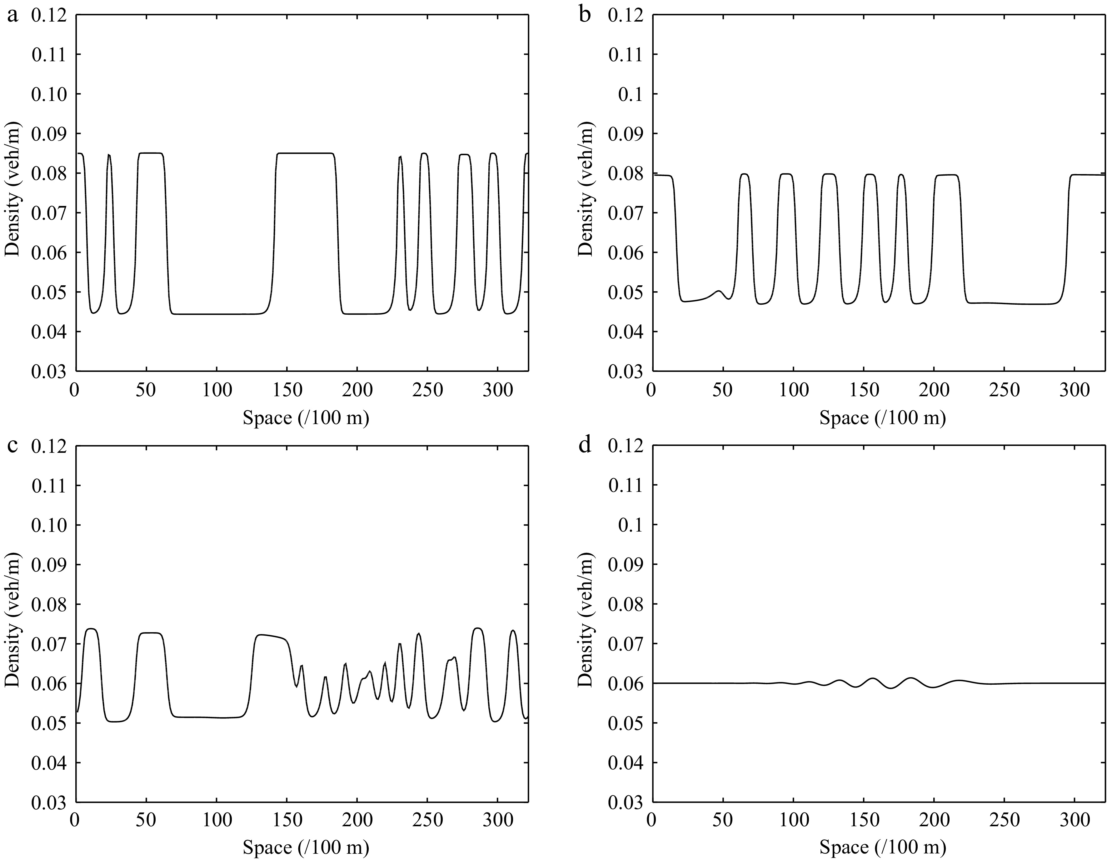
Figure 13.
Instantaneous density distribution of traffic flow corresponding to Fig. 12 at t = 3,000 s.
-
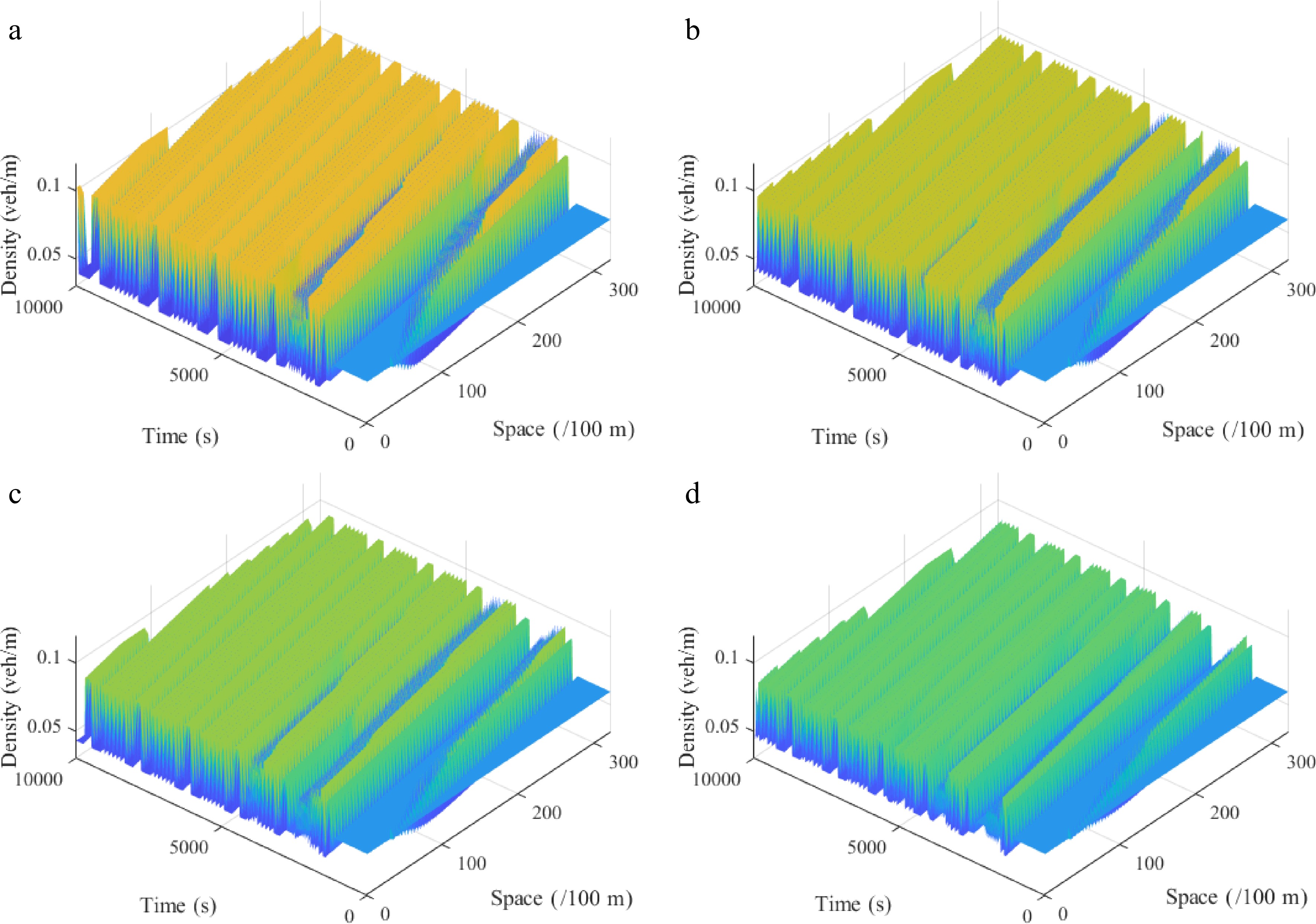
Figure 14.
Spatiotemporal diagram of density waves affected by the initial disturbance corresponding to different values of parameter l under the uphill scenario, where: (a) l = 0; (b) l = 1; (c) l = 2; (d) l = 3. (
$ {\rho _0} $ $ \theta $ $ r $ -
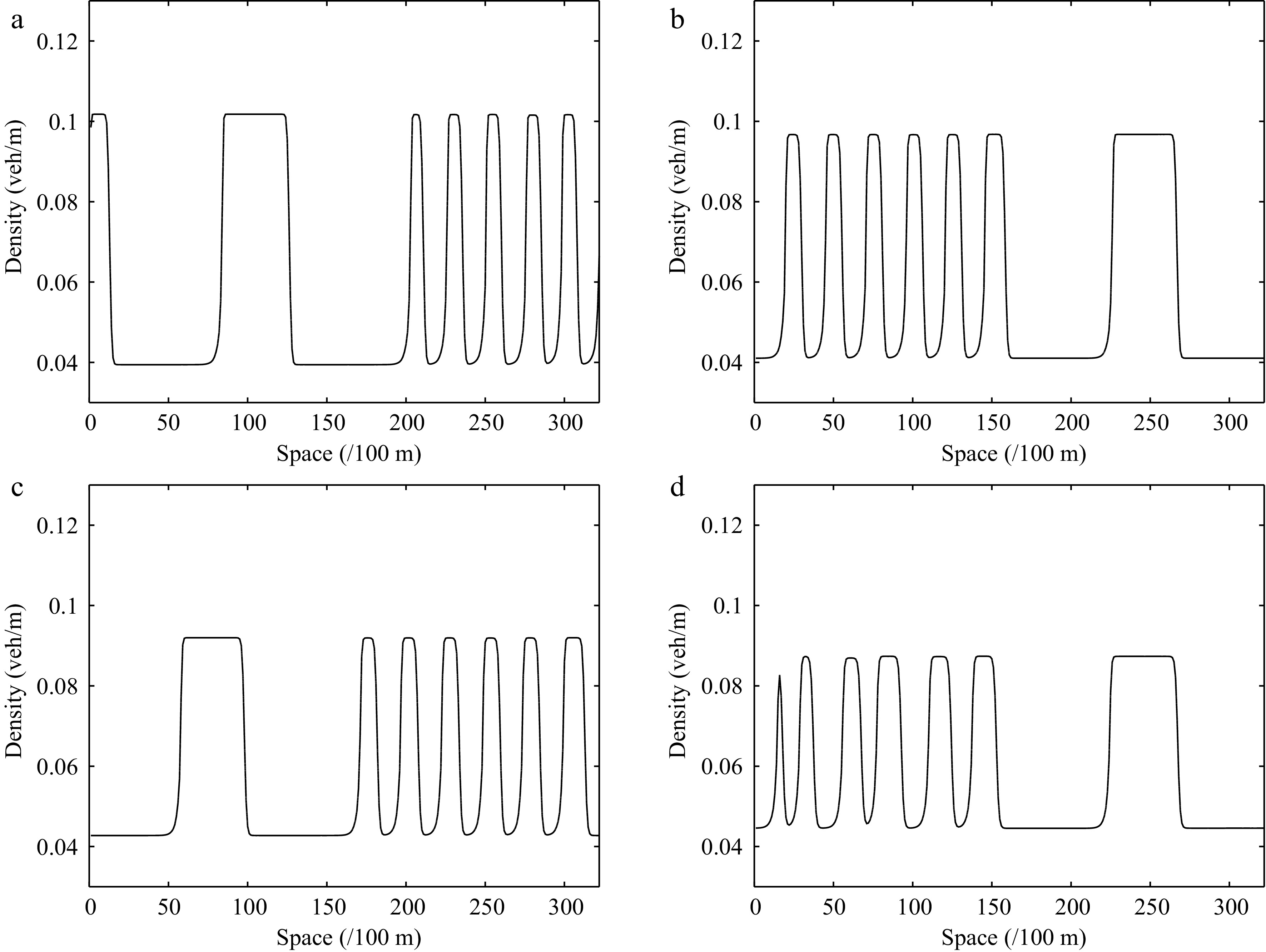
Figure 15.
Instantaneous density distribution of traffic flow corresponding to Fig. 14 at t = 3,000 s.
-
Authors Characteristics References Mohan R, Chen R Heterogeneous traffic flow [25−27] Lu S Higher-order [28,29] Liu H, Cheng R Traffic jerk effect [30,31] Hao L, Yu L. Delay effect [32,33] Liu Z, Zhai C Taillight effect [34,35] Jiao Y, Zhai C Backward looking effect [36,37] Cheng R, Zhai Q Memory effect [38−40] Cheng R, Wang Z Driver's characteristics [41,42] Zhai C, Chen J Slope road / Gradient highways [43,44] Xue Y, Liu Z Curved road [45,46] Guan X, Peng G Anticipation effect [47,48] Ngoduy D, Bouadi M Stochastic continuum models [49,50] Wang Z, Tang T Driver’s bounded rationality [51,52] Table 1.
Representative literature on continuum models.
-
Symbols Definition n The subscript of vehicles a Driver's sensitivity $ {v_n} $ The instantaneous velocity of vehicle n $ \Delta {x_n} $ The instantaneous headway of vehicle n $ {V^{op}}( \cdot ) $ Optimal velocity function $ {v_{\max }} $ The maximum allowable driving velocity under regular road scenes $ {y_s} $ Safety distance without collisions under regular road scenes $ \lambda $ Sensitivity coefficient of the velocity difference $ H( \cdot ) $ Heaviside function $ {s_n} $ Instantaneous position information of vehicle n on the gyroidal road, and $ {s_n} = r \times {\varphi _n} $ $ \Delta {s_n} $ Instantaneous headway information of vehicle n on the gyroidal road, and $ \Delta {s_n} = r \times \Delta {\varphi _n} $ $ r $ The radius of curvature, where $ r = {\gamma \mathord{\left/ {\vphantom {\gamma {\cos \theta }}} \right. } {\cos \theta }} $ $ \gamma $ The radius of the circle $ \theta $ Slope angle, $ \theta < 0 $ $ \theta > 0 $ $ V( \cdot ) $ Optimal speed function on the gyroidal road $ {\omega _{\max }} $ The maximum allowable angular velocity on gyroidal roads $ {y_s}\left( \theta \right) $ The minimum allowable safety distance on gyroidal roads, where $ {y_s}\left( \theta \right) = {y_s}\left( {1 - \alpha \sin \theta } \right) $ $ \alpha $ Is a constant. Here, we set it as $ \alpha = 1 $ $ {v_{g,\max }} $ Maximum reduced or enhanced speed on the gyroidal road, to simplify the calculation, we set $ {v_{g,\max }} = \sin \theta $ $ m $ The mass of vehicles $ g $ Gravitational acceleration information, where we set g = 9.8 m·s−1 $ \mu $ Lateral friction coefficient $ k $ The adjustment coefficient; here k = 0.1 $ l $ The number of vehicles ahead considered Table 2.
Primary notations used in the proposed model.
-
Parameter Value Unit vf 30 m/s L 20 km cm 11 − ρm 0.2 veh/m a 0.3 s−1 λ 0.3 − k 0.1 − g 9.8 m/s2 r 60 m l 3 − ∆t 1 s ∆x 100 m Table 3.
Parameter settings corresponding to Case I.
-
Parameter Value Unit vf 30 m/s L 32.2 km ρm 0.2 veh/m a 0.34 s−1 λ 0.3 − k 0.1 − g 9.8 m/s2 ∆t 1 s ∆x 100 m Table 4.
Parameter settings.
Figures
(15)
Tables
(4)