A comparative study of GA, PSO and SCE algorithms for estimating kinetics of biomass pyrolysis

Hongfang Wang; Junhui Gong; Hongfang Wang; Junhui Gong

doi:10.48130/EMST-2023-0009

Figures (12) Tables (4)

Figure 1.
Dependencies of (a) mass and (b) MLR of beech wood on temperature at different heating rates.
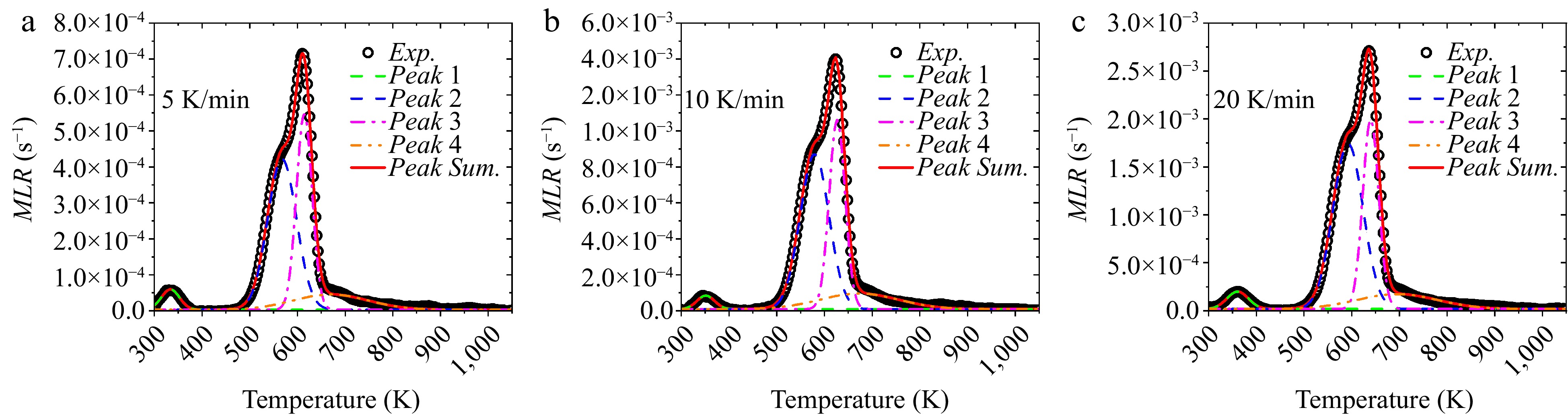
Figure 2.
Separated MLR curves using Gauss multi-peak fitting method at different heating rates.
Figure 3.
Linear fittings of ${\text{ln}}( {\beta /{T_p}^2} )$ vs $1/{T_p}$ in the Kissinger method.
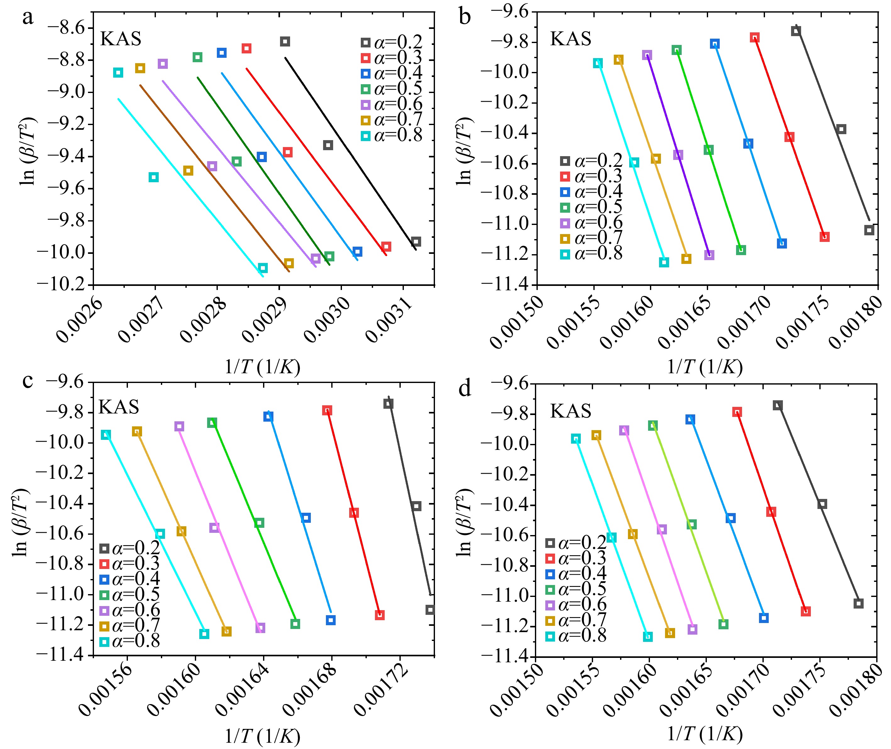
Figure 4.
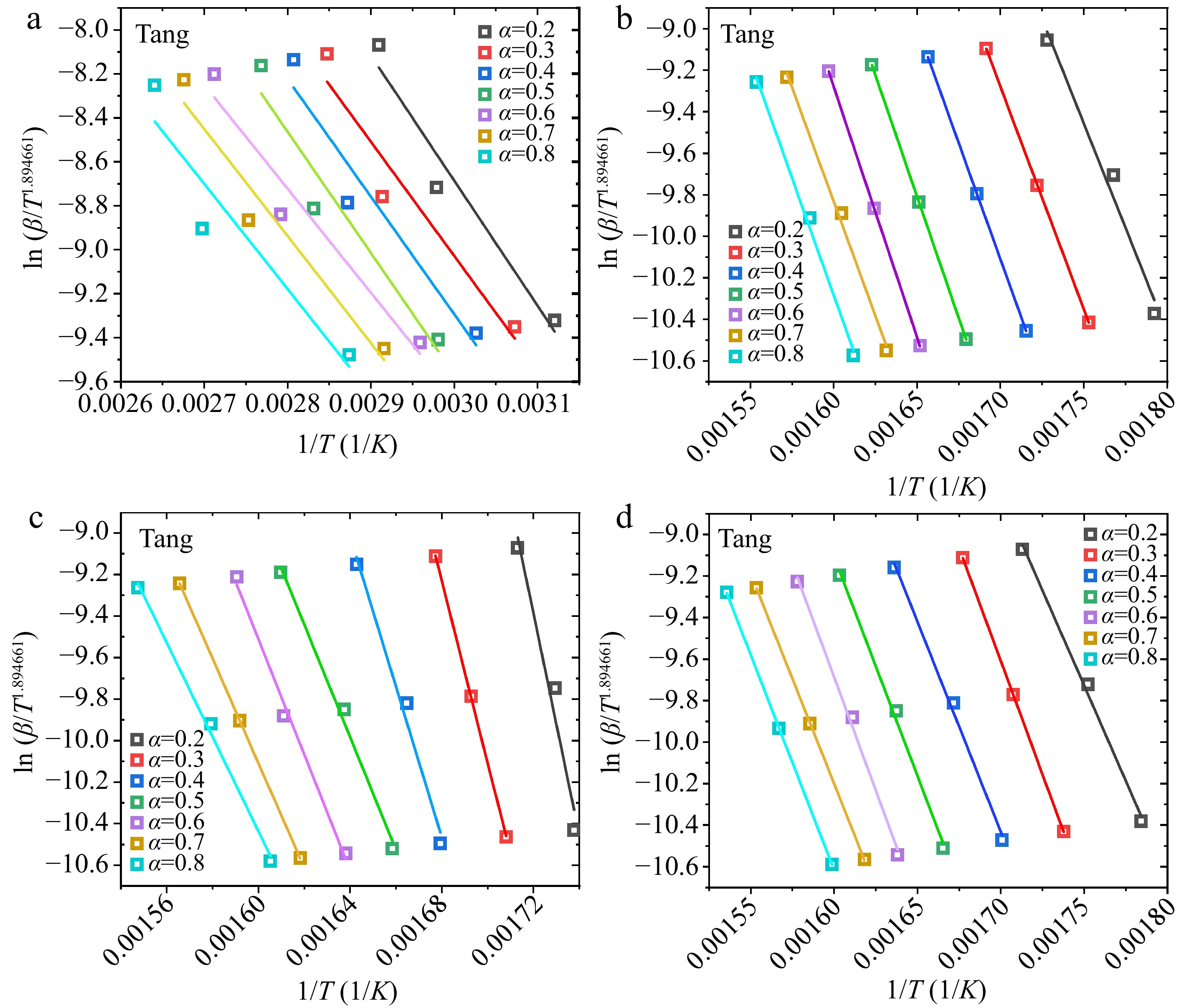
Linear fittings of ${\text{ln}}( {\beta /{T^2}} )$ vs $1/T$ plots in the KAS method: (a) water, (b) hemicellulose, (c) cellulose, (d) lignin.
Figure 5.
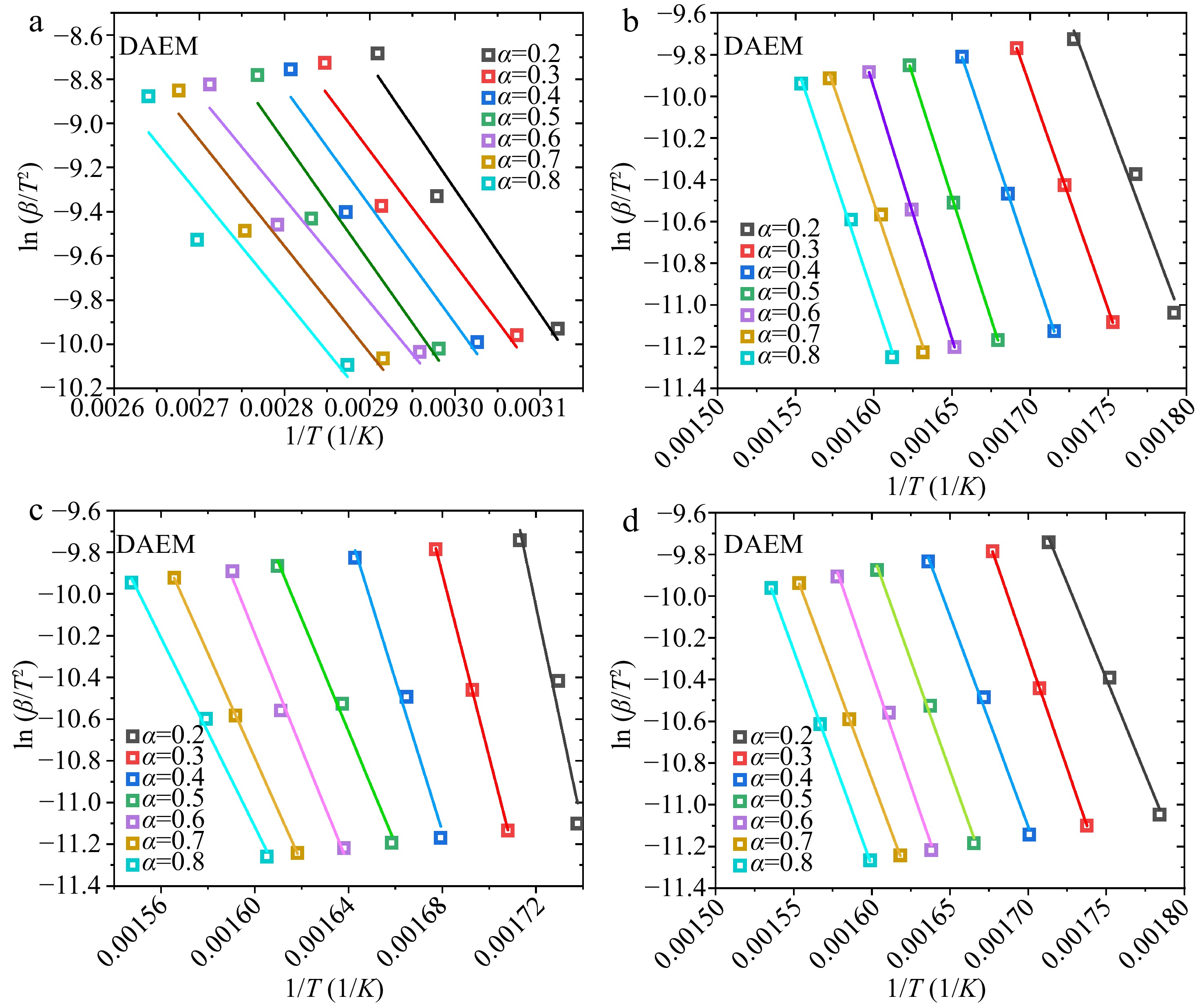
Linear fittings of $\ln ( {\beta /{T^{1.894661}}} )$ vs $1/T$ plots in the Tang method: (a) water, (b) hemicellulose, (c) cellulose, (d) lignin.
Figure 6.
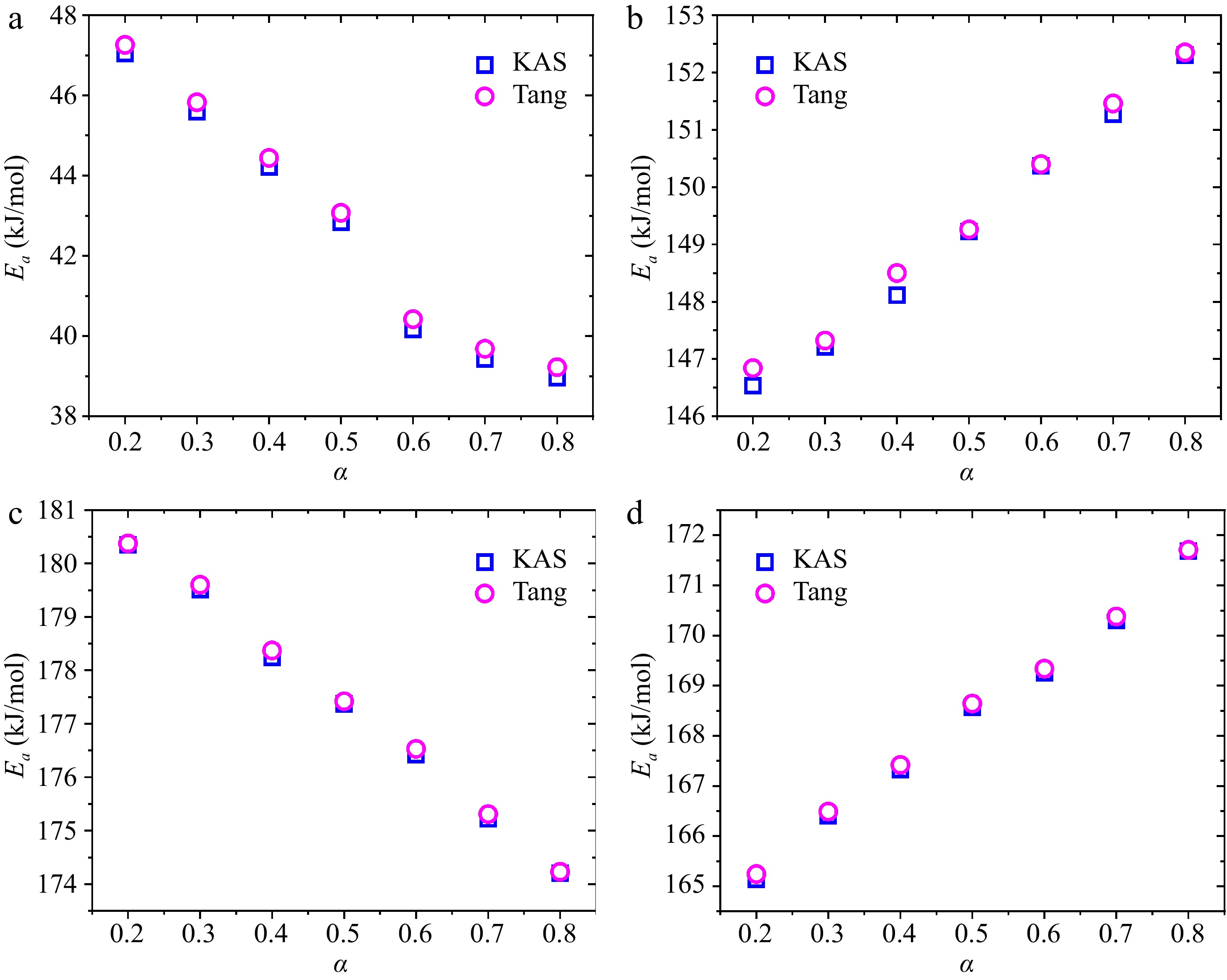
Linear fittings of ${\text{ln}}( {\beta /{T^2}} )$ vs $1/T$ plots in the DAEM method: (a) water, (b) hemicellulose, (c) cellulose, (d) lignin.
Figure 7.
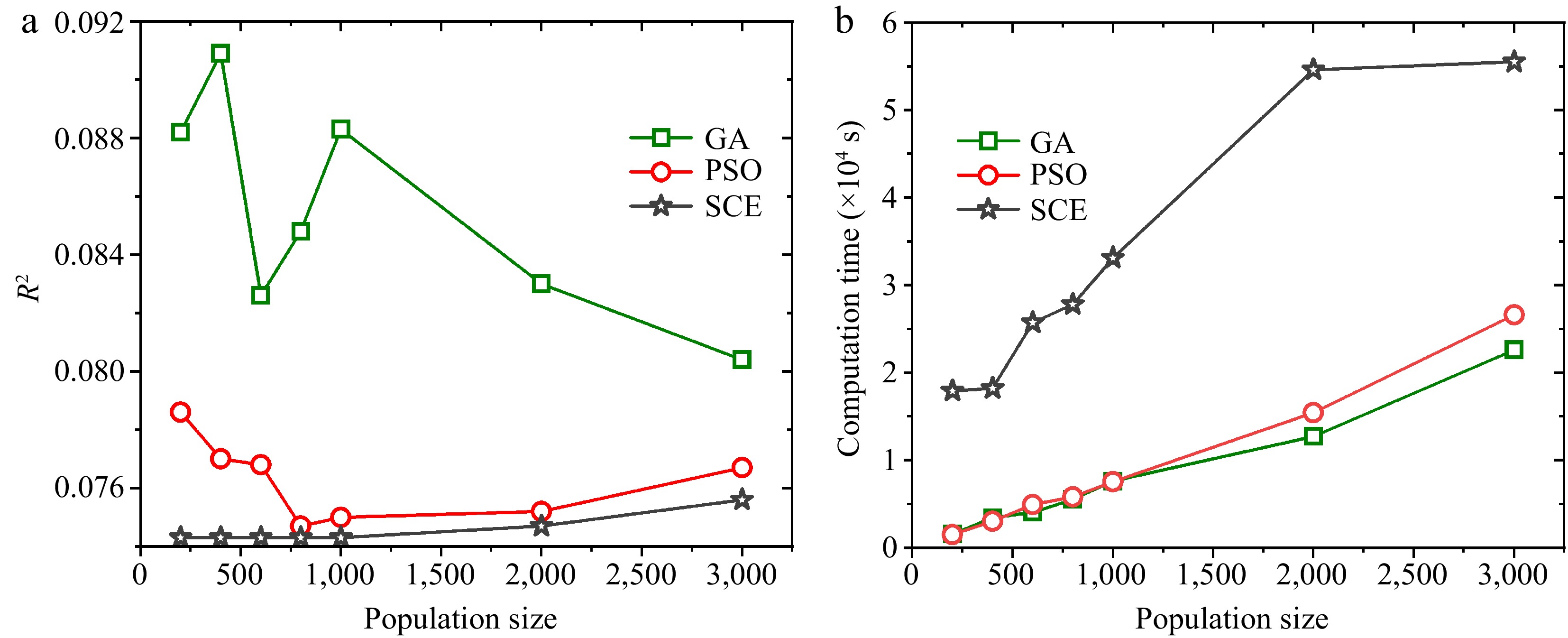
Dependencies of calculated ${E_a}$ on α using the KAS and Tang methods: (a) water, (b) hemicellulose, (c) cellulose, (d) lignin.
Figure 8.
Objective function values and the computation times of the three algorithms when optimizing kinetics of wood pyrolysis with 200-3000 population sizes and 200 iterations.
Figure 9.
Objective function value evolutions of the three algorithms when optimizing kinetics of wood pyrolysis with 3,000 population size and 6,000 iterations.
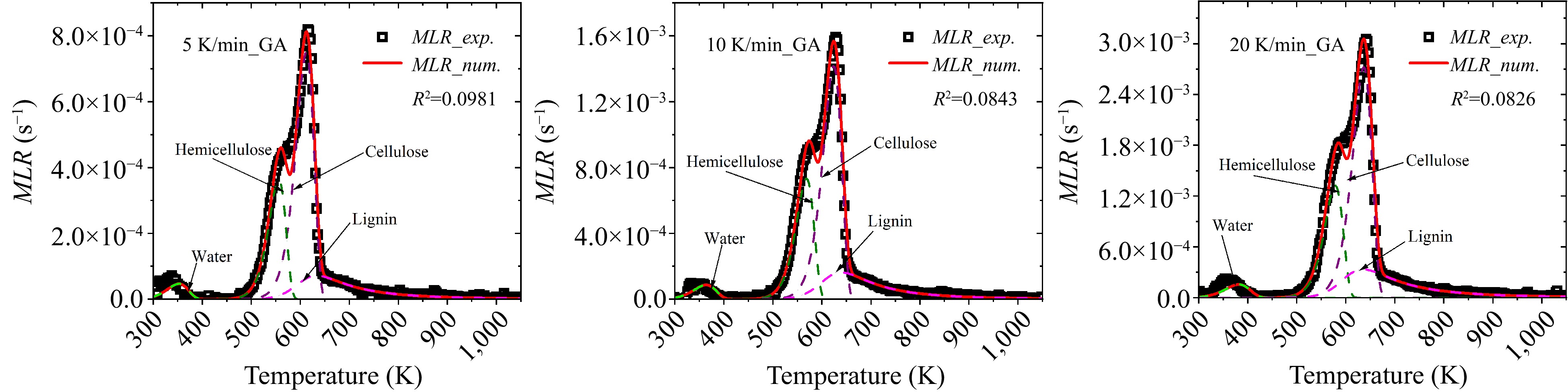
Figure 10.
Comparison between experimental and numerical MLRs using optimized parameters of GA at 5, 10 and 20 K/min heating rates.
Figure 11.
Comparison between experimental and numerical MLRs using optimized parameters of PSO at 5, 10 and 20 K/min heating rates.
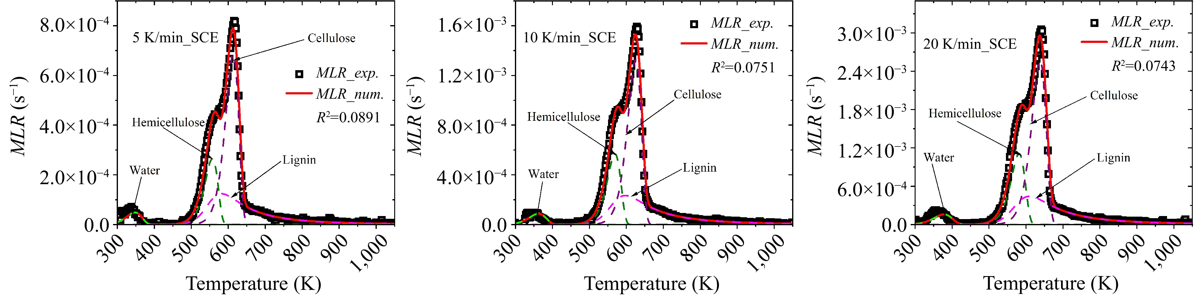
Figure 12.
Comparison between experimental and numerical MLRs using optimized parameters of SCE at 5, 10 and 20 K/min heating rates.
# Reaction

1 Water → Vapor
2 Hemicellulose → θ₁ Char + (1−θ₁) Gas_H
3 Cellulose → θ₂ Char + (1−θ₂) Gas_C
4 −Lignin → θ₃ Char + (1-θ₃) Gas_L

Table 1.
Reaction mechanism of beech wood.

Component	Kissinger		KAS		Tang		DAEM		Average
Component	A	E_a	A	E_a	A	E_a	A	E_a	A	E_a
Water	1.49 × 10³	44.8	1.01 × 10³	42.6	2.61 × 10³	42.9	1.53 × 10³	42.6	1.72 × 10³	42.7
Hemicellulose	1.12 × 10¹²	147.8	1.30 × 10¹³	144.7	3.06 × 10¹³	154.9	9.31 × 10¹²	144.7	1.77 × 10¹³	148.1
Cellulose	4.09 × 10¹²	166.3	4.70 × 10¹²	174.8	4.84 × 10¹²	169.7	4.12 × 10¹²	174.8	4.55 × 10¹²	173.1
Lignin	2.34 × 10¹¹	180.5	6.40 × 10¹¹	170.7	1.46 × 10¹²	171.2	7.96 × 10¹¹	170.7	9.66 × 10¹¹	170.9

Table 2.

Estimated $A$ (s⁻¹) and ${E_a}$ (kJ/mol) of wood pyrolysis by the Kissinger, KAS, Tang, and DAEM methods.

Population size	GA		PSO		SCE
Population size	t_com × 10⁴ (s)	R² × 10⁻²	t_com × 10⁴ (s)	R² × 10⁻²	t_com × 10⁴ (s)	R² × 10⁻²
200	0.16	8.82	0.15	7.86	1.79	7.43
400	0.34	9.09	0.30	7.70	1.82	7.43
600	0.40	8.26	0.49	7.68	2.57	7.43
800	0.55	8.48	0.58	7.47	2.78	7.43
1,000	0.76	8.83	0.75	7.50	3.31	7.43
2,000	1.27	8.30	1.54	7.52	5.46	7.47
3,000	2.26	8.44	2.66	7.67	5.55	7.56

Table 3.

Computation times and ${R^2}$ of GA, PSO and SCE optimizations.

Component	Parameter	Search range	GA	PSO	SCE
Water	A (s⁻¹)	1.72 × 10²−1.72 × 10⁴	1.47 × 10⁴	1.49 × 10⁴	1.49 × 10⁴
Water	E_a (kJ/mol)	4.28 × 10⁴−4.48 × 10⁴	4.4 × 10⁴	4.4 × 10⁴	4.4 × 10⁴
Hemicellulose	A (s⁻¹)	9.41 × 10¹¹−9.41 × 10¹³	5.53 × 10¹²	4.49 × 10¹²	4.18 × 10¹²
	E_a (kJ/mol)	1.38 × 10⁵−1.58 × 10⁵	1.4 × 10⁵	1.38 × 10⁵	1.38 × 10⁵
	θ	0−0.5	0.28	0.38	0.37
Cellulose	A (s⁻¹)	4.32 × 10¹¹−4.32 × 10¹³	4.09 × 10¹²	3.95 × 10¹²	4.09 × 10¹²
	E_a (kJ/mol)	1.6 × 10⁵−1.8 × 10⁵	1.63 × 10⁵	1.63 × 10⁵	1.64 × 10⁵
	θ	0−0.5	0.13	0.12	0.12
Lignin	A (s⁻¹)	6.0 × 10¹⁰−6.0 × 10¹²	2.22 × 10¹¹	1.96 × 10¹¹	1.15 × 10¹¹
	E_a (kJ/mol)	0−3.0 × 10⁵	1.23 × 10⁵	1.16 × 10⁵	1.13 × 10⁵
	θ	0−1	0.14	0.01	0.01
	n	0−5	4.67	4.99	5

Table 4.

Best optimized kinetics of wood pyrolysis by GA, PSO and SCE.

#	Reaction
1	Water → Vapor
2	Hemicellulose → θ₁ Char + (1−θ₁) Gas_H
3	Cellulose → θ₂ Char + (1−θ₂) Gas_C
4	−Lignin → θ₃ Char + (1-θ₃) Gas_L