-
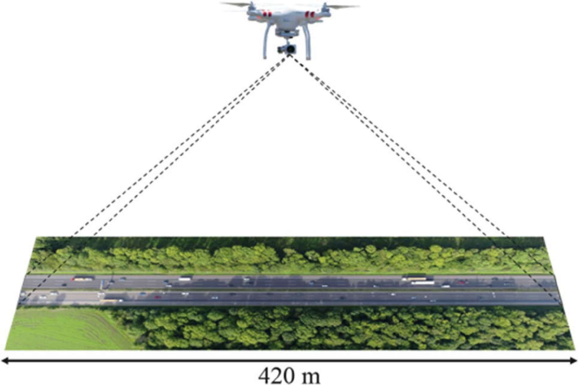
Figure 1.
A drone recording the motion of vehicles along a 420-meter stretch of highway from an overhead perspective[38].
-

Figure 2.
The illustration of spatial range from a top view.
-
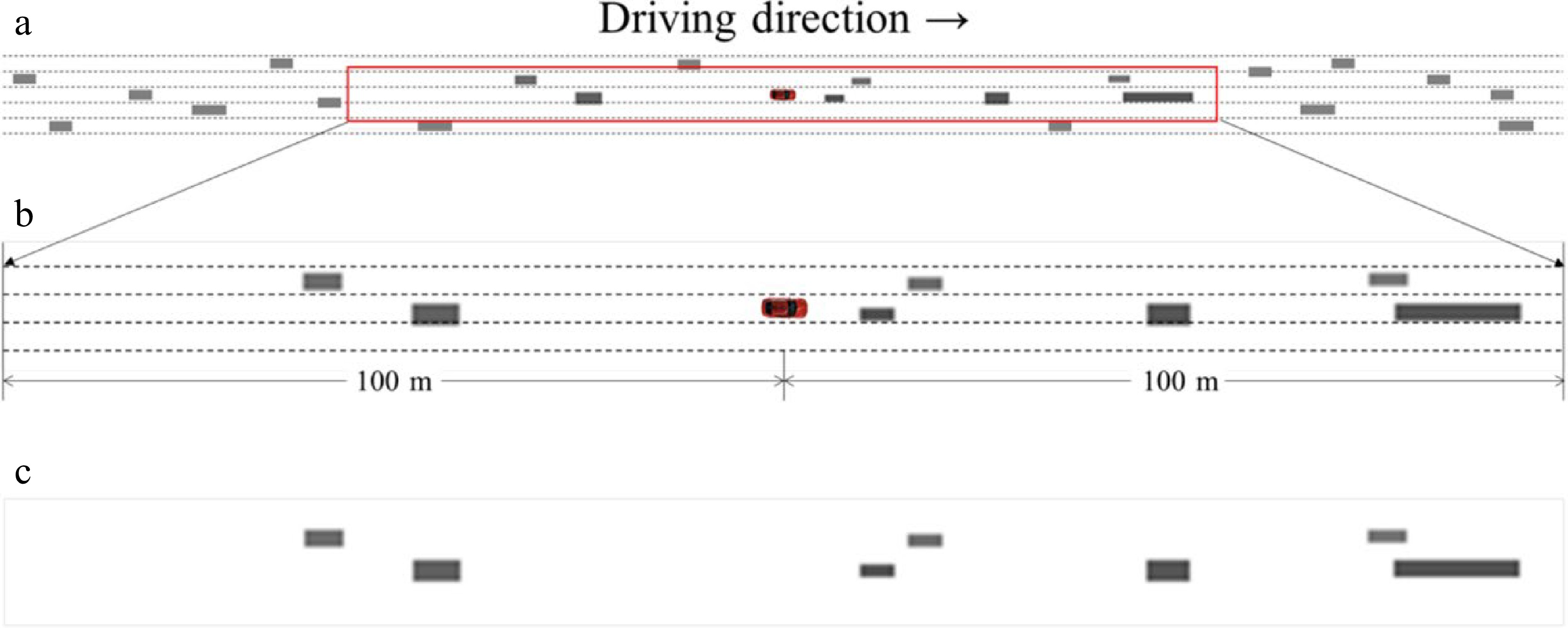
Figure 3.
The detailed and simplified top views for each moment with the subject vehicle in the center. (a) is an illustration of the spatial range, (b) is a zoomed-in version of the study area, and (c) is a simplified version as input to the model.
-
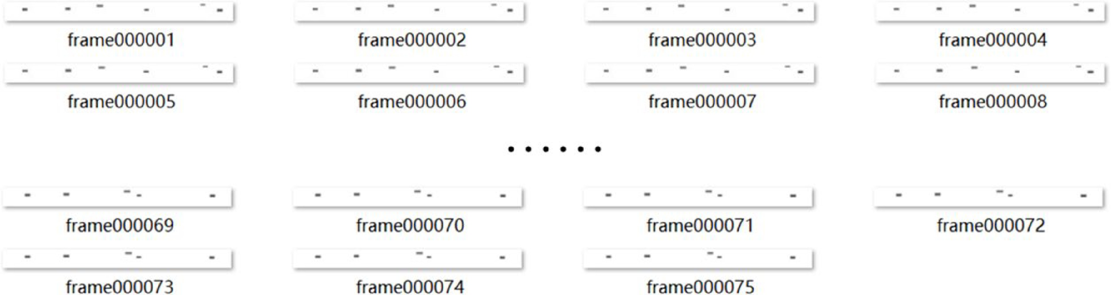
Figure 4.
The time series top view set describing an event.
-
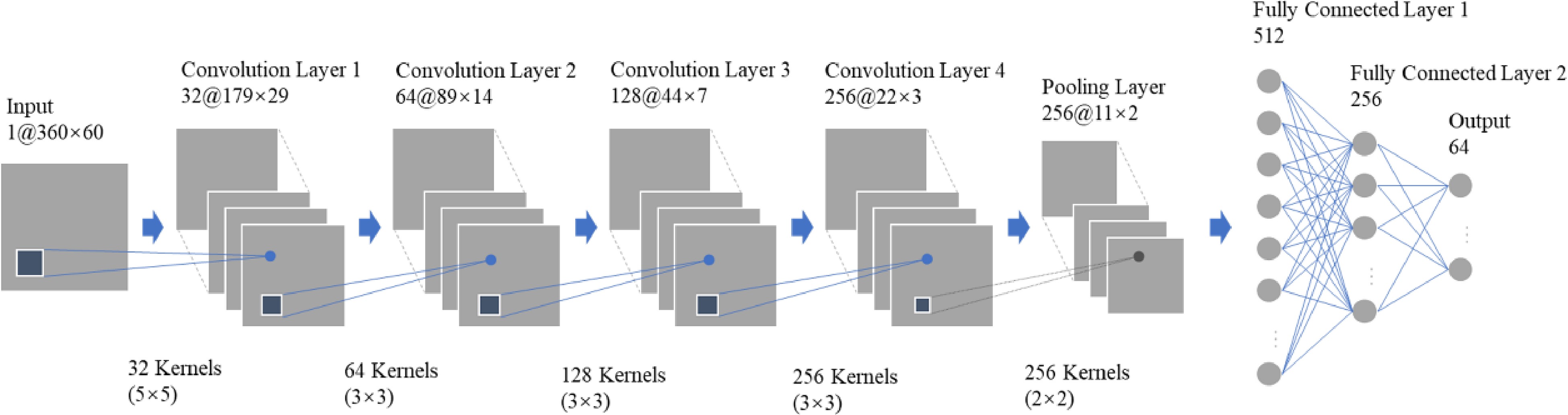
Figure 5.
The structure of CNN model.
-
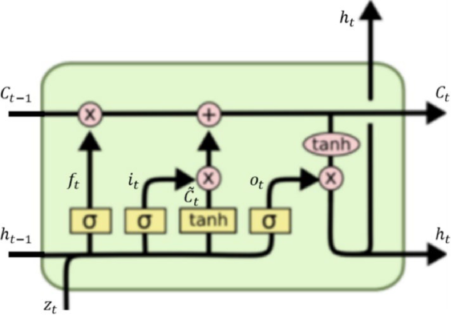
Figure 6.
The basic unit of LSTM model[43].
-
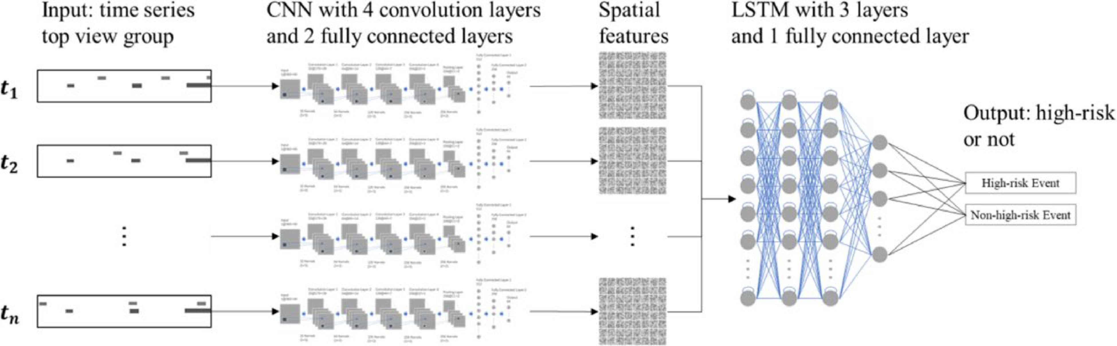
Figure 7.
The proposed CNN-LSTM model.
-
Modeling process Parameters with values Input of CNN 75 top views with both the front and rear of the subject vehicle: 360 × 30
(or 75 top views with only the front of the subject vehicle: 360 × 60)Convolution layer No. of layers: 4
No. of kernels: 32, 64,128, and 256
Kernel size: (5 × 5), (3 × 3), (3 × 3), and (3 × 3)
Stride: (2,2), (2,2), (2,2), and (2,2)
Padding: (0,0), (0,0), (0,0), and (0,0)
Activating function: ReLUPooling layer No. of layers: 1
Kernel size: (2 × 2)
Stride: (2,2)
Padding: (0,0)Fully connected layer No. of layers: 2
Hidden neurons: 512 and 256
Activating function: ReLUOutput of CNN model/ Input of LSTM model No. of features: 64 (for each top view)
75 top views for each eventLSTM No. of layers: 3
Hidden neurons: 512, 512, 512Fully connected layer No. of layers: 1
Hidden neurons: 256
Activating function: ReLUOutput of LSTM model Binary classification result: high-risk or non-high-risk Training process Backpropagation
Learning rate: StepLR (lr = 1e-3, γ = 0.3)
Loss function: Cross-entropy
Mini-batch size: 128
Epochs: 50Table 1.
Parameters with values in the CNN-LSTM modeling process.
-
Actual condition Predicted condition Positive Negative Positive True Positive (TP) False Negative (FN) Negative False Positive (FP) True Negative (TN) Table 2.
The confusion matrix.
-
Spatial range Temporal range 1 100 m in both the front and rear of the subject vehicle 5 s to 2 s before the zero time 2 5 s to 3 s before the zero time 3 4 s to 2 s before the zero time 4 Only 100 m in the front of the subject vehicle 5 s to 2 s before the zero time 5 5 s to 3 s before the zero time 6 4 s to 2 s before the zero time Table 3.
Descriptions of the six experiment designs.
-
Sensitivity False Alarm Rate AUC 1 0.988 0.177 0.992 2 0.977 0.119 0.988 3 0.988 0.274 0.989 4 0.996 0.065 0.997 5 0.992 0.032 0.996 6 0.988 0.387 0.988 Table 4.
The prediction performances of the six experiment designs.
-
Loss and accuracy ROC curve 1 

2 

3 

4 

5 

6 

Table 5.
The loss, accuracy, and ROC curve of the six experimental designs.
-
Table 6.
Comparation results of modeling performance based on testing data.
Figures
(7)
Tables
(6)