-
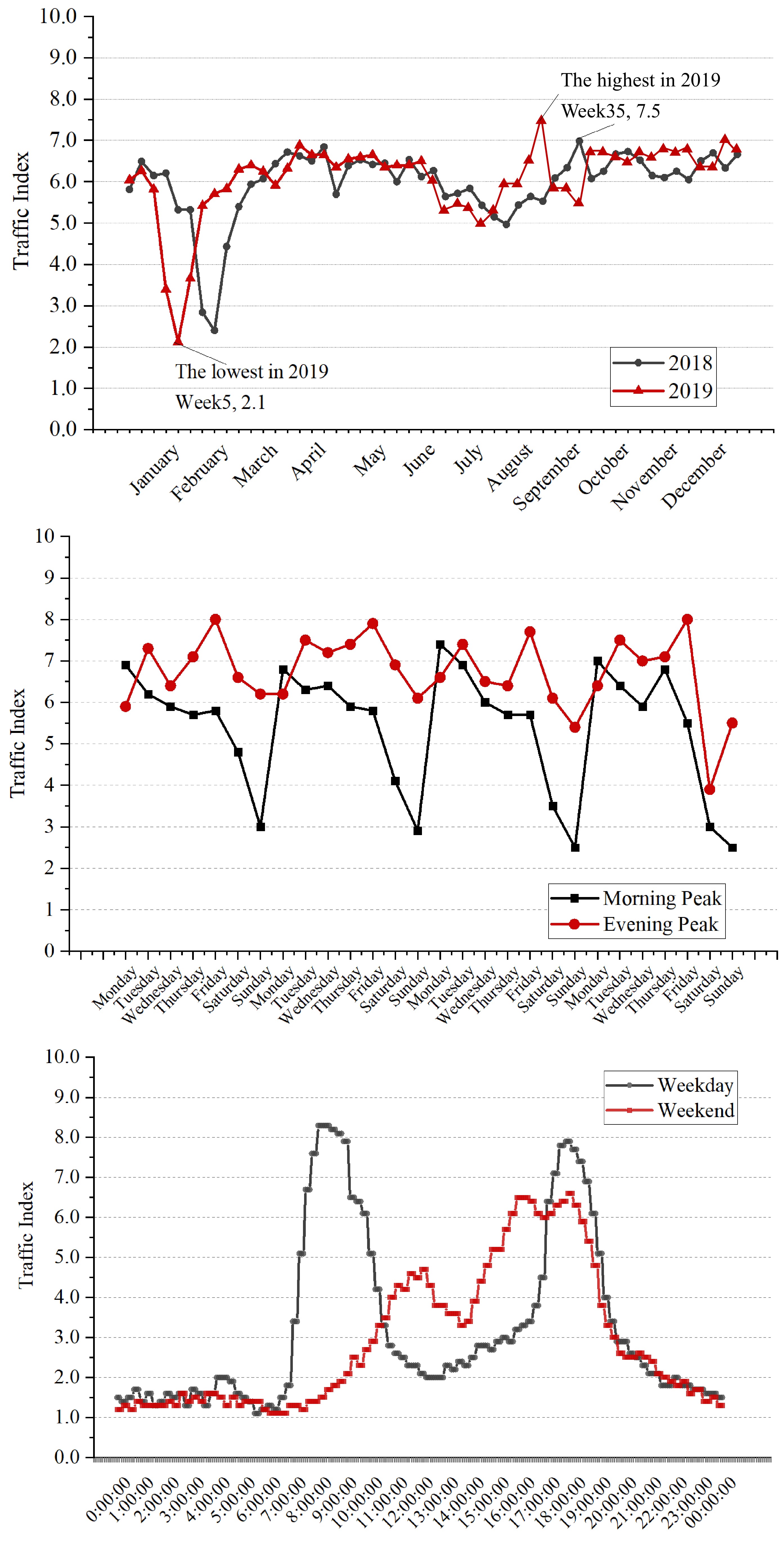
Figure 1.
Fluctuation characteristics of TPI over different periods.
-
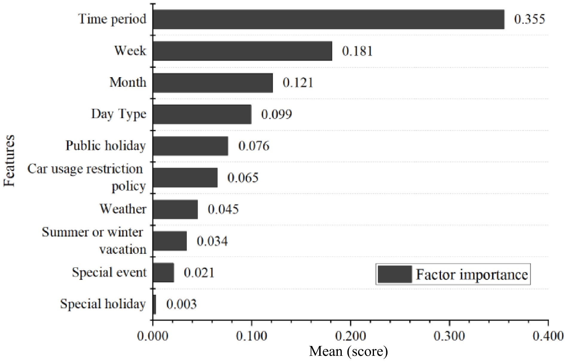
Figure 2.
Relative importance of different influencing factors.
-
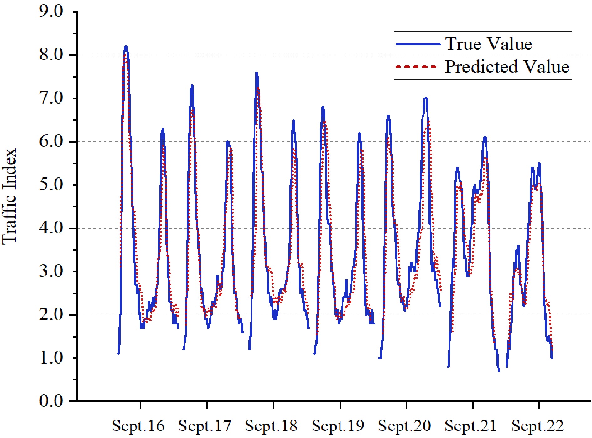
Figure 3.
Comparison of TPI prediction results for one week.
-
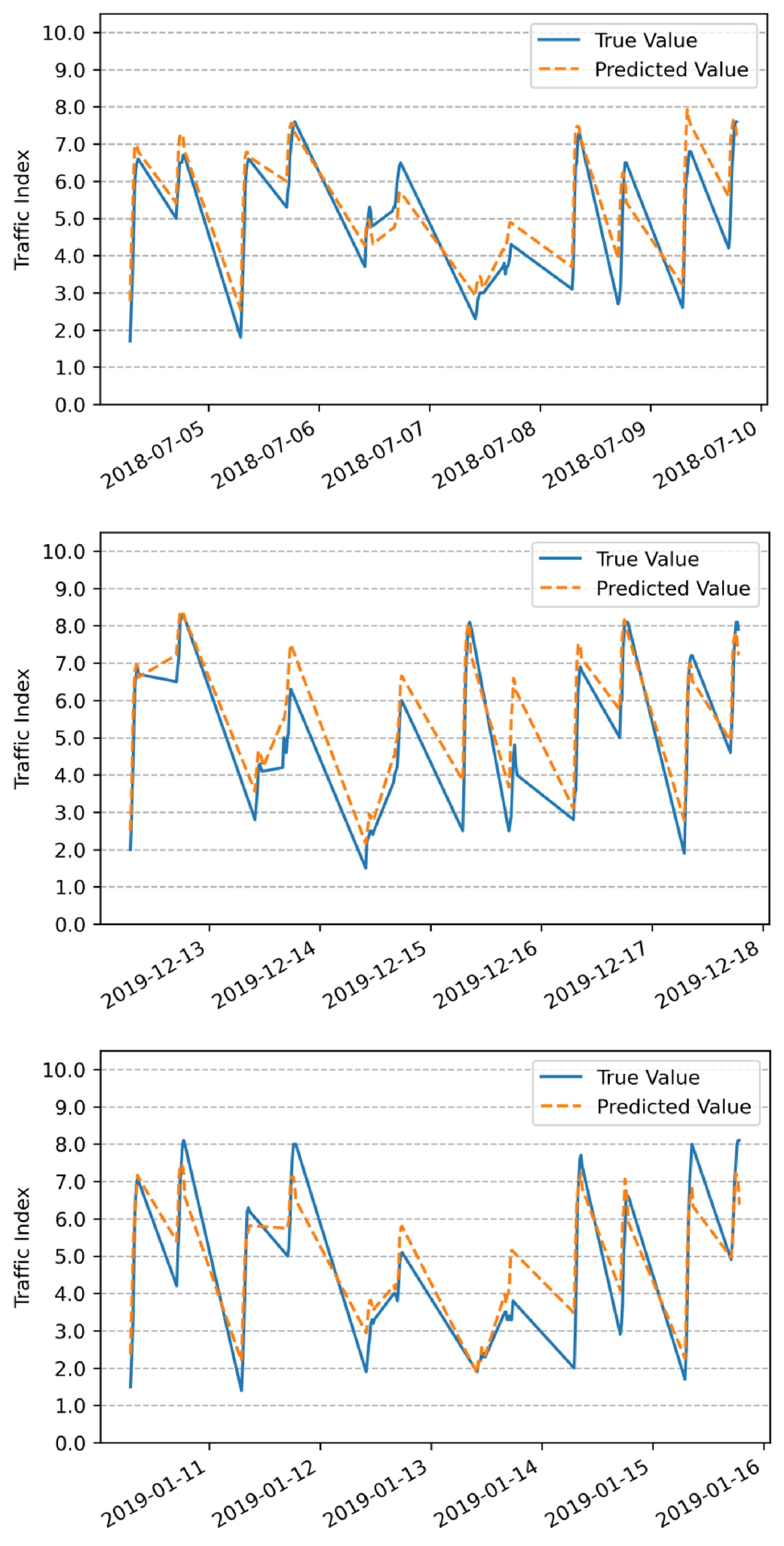
Figure 4.
Comparison of TPI prediction results for rainy, snowy, and hazy weather.
-
Name Symbol Count Month 0: January; 1: February; ...; 11: December 18 months Week 0: Sunday; 1: Monday; ...; 6: Saturday 72 weeks Time period 21:0500-0515; 22:0515-0530; ...; 92:2245-2300 39,312 periods Day type 0: Weekday; 1: Weekend 546 d Public holiday 1: First day of holiday 12 d 2: Middle day(s) during holiday 25 d 3: Last day of holiday 12 d Summer or
winter vacation0: Normal days 426 d 1: Summer and winter vacation 120 d Special holiday 0: Normal day 421 d 1: Special holiday 5 d Car usage
restriction policy0: The last digit of license plate number is 0 or 5. 73 d 1: The last digit of license plate number is 1 or 6. 74 d 2: The last digit of license plate number is 2 or 7. 73 d 3: The last digit of license plate number is 3 or 8. 71 d 4: The last digit of license plate number is 4 or 9. 70 d 5: No limit 185 d Weather 0: Sunny, or cloudy
1: Rain490 d 63 d 2: Snow 6 d 3: Haze 31 d Special events 1: Short-term events 252 times 2: Large events lasting the whole day 314 times Table 1.
Descriptive statistics of influencing factors.
-
XGBoost Pseudo-code: Input: Training set D = {(xi, yi)}, where xi represents the i-th input vector and yi is the corresponding label.
Output: Prediction model f(x).// Step 1: Initialize the ensemble
Initialize the base prediction model as a constant value: f0(x) = initialization_constant// Step 2: Iterate over the boosting rounds
for m = 1 to M: // M is the number of boosting rounds// Step 3: Compute the pseudo-residuals
Compute the negative gradient of the loss function with respect to the current model's predicted values:
rmi = - ∂L(yi, fm−1(xi)) / ∂fm−1(xi)// Step 4: Fit a base learner to the pseudo-residuals
Fit a base learner (e.g., decision tree) to the pseudo-residuals: hm(x).// Step 5: Update the prediction model
Update the prediction model by adding the new base learner:
fm(x) = fm−1(x) + η * hm(x), where η is the learning rate.// Step 6: Output the final prediction model
Output the final prediction model: f(x) = fm(x)Table 2.
The pseudo-code of XGBoost algorithm.
-
Learning rate The number of trees R2 MAE MSE Maxmium depth of the tree = 3 0.05 1,400 0.8800 0.4934 0.4911 0.1 1,300 0.8779 0.4978 0.4998 0.5 160 0.8666 0.5274 0.5461 1 140 0.8117 0.6442 0.7708 Maxmium depth of the tree = 4 0.05 700 0.8797 0.4923 0.4927 0.1 600 0.8978 0.4640 0.4430 0.5 120 0.8872 0.4763 0.4620 1 110 0.8889 0.4791 0.4550 Maxmium depth of the tree = 5* 0.05 350 0.8865 0.4734 0.4646 0.1* 160* 0.8950 0.4474 0.4309 0.5 50 0.8886 0.4730 0.4560 1 30 0.8756 0.5103 0.5095 Maxmium depth of the tree = 6 0.05 195 0.8896 0.4655 0.4520 0.1 70 0.8791 0.4902 0.4950 0.5 30 0.8945 0.4572 0.4321 1 20 0.8860 0.4838 0.4666 Table 3.
Performance of extreme gradient boosting (XGBoost) models for daily TPI prediction.
-
Forecast data Prediction accuracy Week 1 (April 22 to April 28, 2019) 94.3% Week 2 (April 29 to May 5 2019) 85.3% Week 3 (May 6 to May 12, 2019) 91.1% Week 4 (May 13 to May 19, 2019) 89.1% Average value 90.0% Table 4.
Forecast accuracy of TPI for each week.
-
TPI prediction Performance of different models
(Measured by MAE, MSE and R2)SVR ElatsicNet Bayesian
RidgeLinear
RegressionXGBoost MAE 0.611 1.668 1.581 2.189 0.396* MSE 1.693 3.111 4.121 3.553 0.989* R2 0.784 0.034 0.113 0.391 0.786* MAE, Mean Absolute Error; MSE, Mean Squared Error Table 5.
Accuracy verification result of different models.
Figures
(4)
Tables
(5)