-
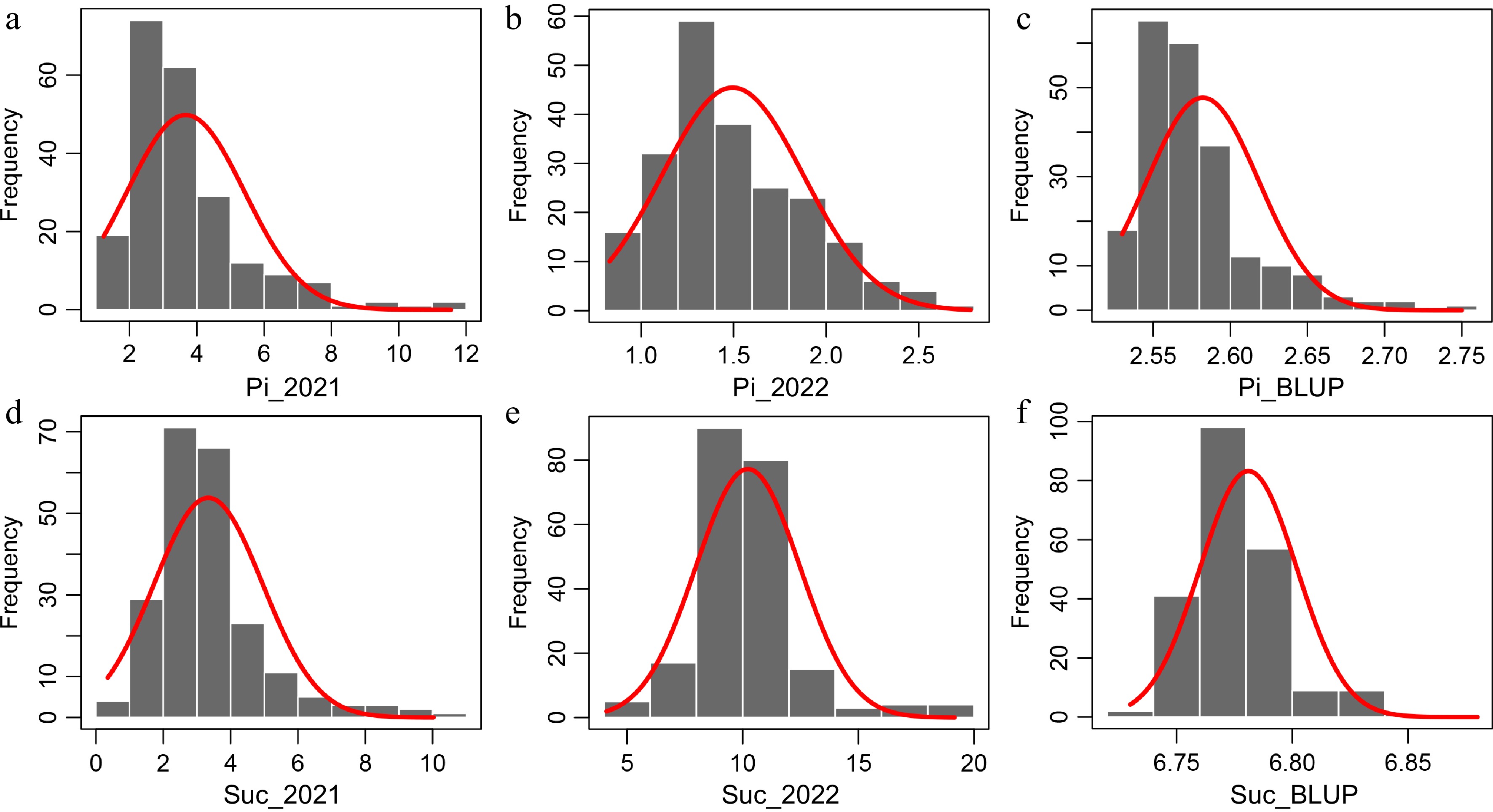
Figure 1.
Frequency distributions of Pi and Suc in the natural population. (a), (b) Frequency distribution of Pi in 2021 and 2022. (c) Frequency distribution of BLUP data for Pi. (d), (e) Frequency distribution of Suc in 2021 and 2022. (f) Frequency distribution of BLUP data for Suc. The curves represent a fit of a normal distribution to the measured distribution.
-
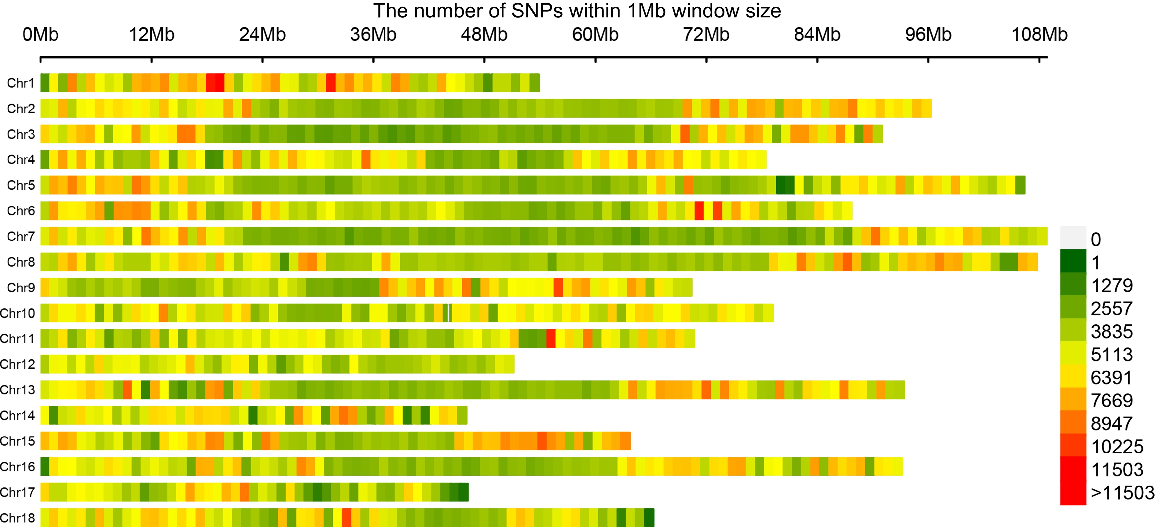
Figure 2.
Genome-wide profiling of SNP density in the natural population. The number of SNPs is counted in 1 Mb intervals, and the color is based on the counted values.
-
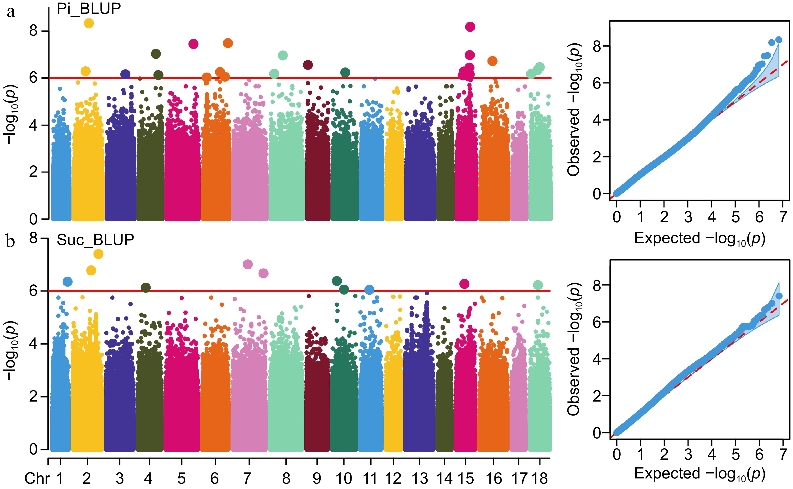
Figure 3.
Manhattan and QQ plots depict the GWAS results of Pi and Suc. (a), (b) GWAS results of Pi and Suc traits using BLUP data. Red lines represent a p-value of 1e-6 and the dot size of significant SNPs is magnified two-fold.
-
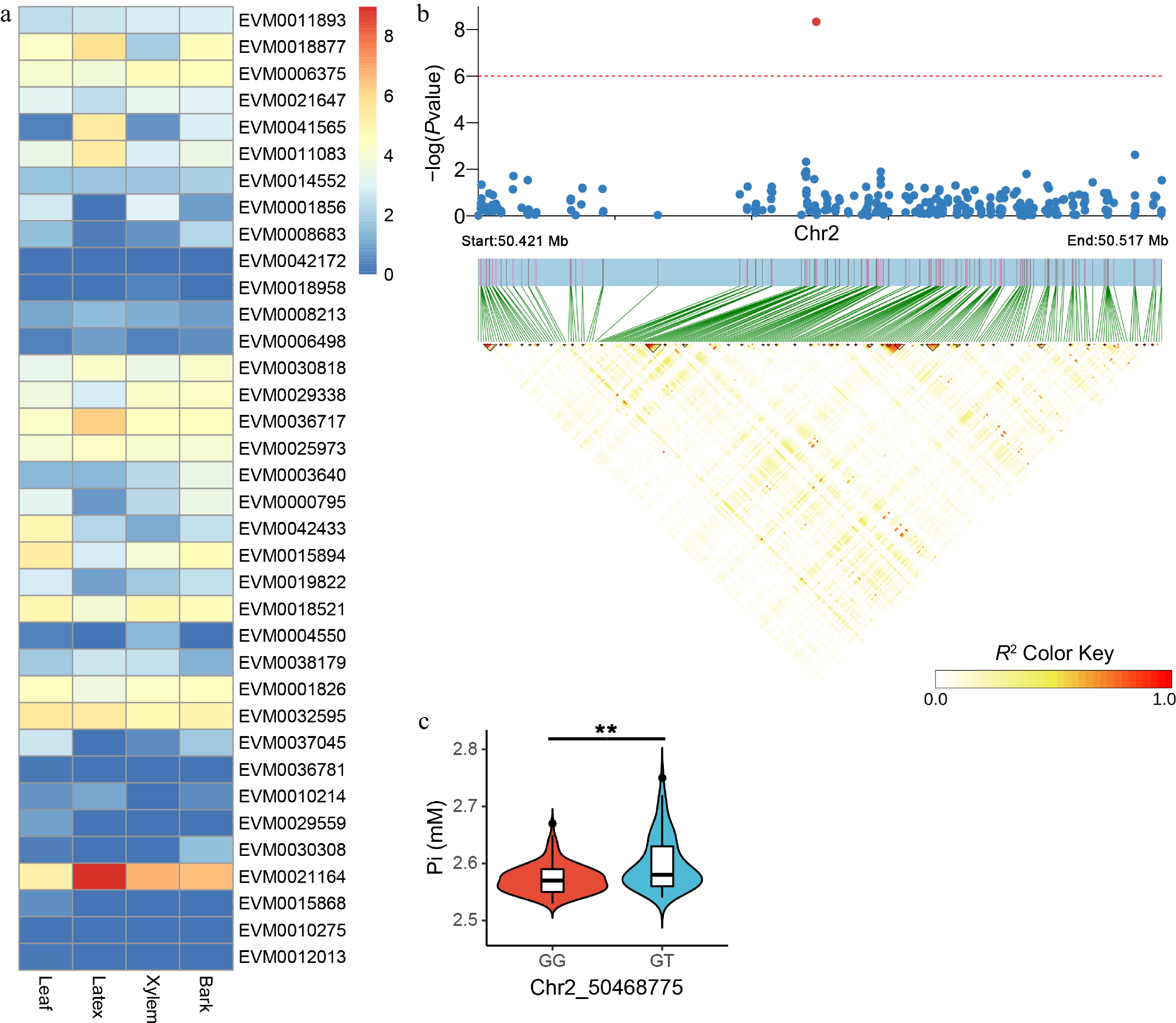
Figure 4.
Candidate gene expression patterns and LD block analysis for Pi-associated variants. (a) Quantification of candidate gene expression levels related to Pi in the leaf, latex, xylem, and bark tissues of RY73397. The color is based on the log2 (FPKM + 1) values. (b) LD block analysis of the most significant SNP correlated with Pi. The red line represents a p-value of 1e-6. (c) Comparison of Pi between GG (n = 143) and GT (n = 75) haplotypes. ** indicates p < 0.01.
-
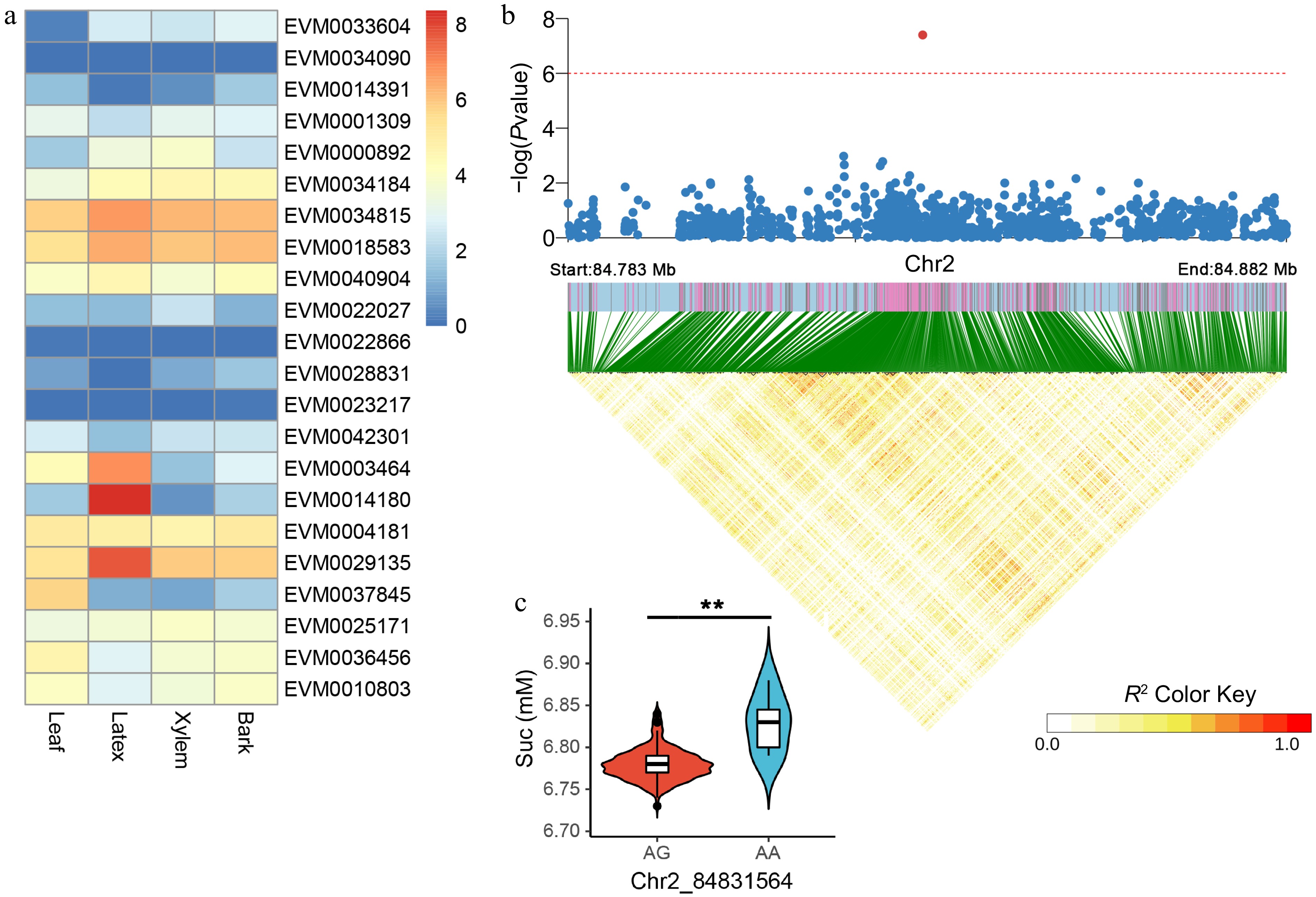
Figure 5.
Candidate gene expression patterns and LD block analysis for Suc-associated variants. (a) Quantification of candidate gene expression levels related to Suc in the leaf, latex, xylem, and bark tissues of RY73397. The color is based on the log2 (FPKM + 1) values. (b) LD block analysis of the most significant SNP correlated with Suc. The red line represents a p-value of 1e-6. (c) Comparison of Suc between AG (n = 212) and AA (n = 6) haplotypes. ** indicates p < 0.01.
Figures
(5)
Tables
(0)