Determining spatial units for modeling regional nonnative invasive plant species spread in the southern US forestlands: using the state of Alabama as an example

Sunil Nepal; Martin A. Spetich; Zhaofei Fan; Sunil Nepal; Martin A. Spetich; Zhaofei Fan

doi:10.48130/forres-0024-0010

Figures (8) Tables (5)

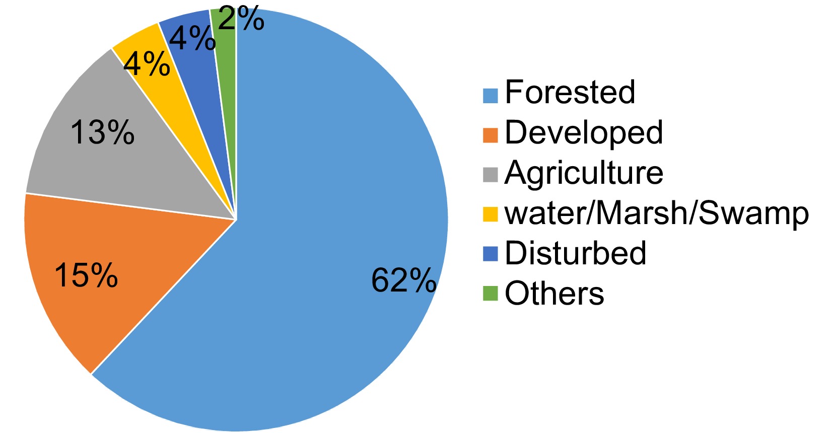
Figure 1.
Land-use in Alabama based on LANDFIRE data (SAF/SRM classes in 2016).
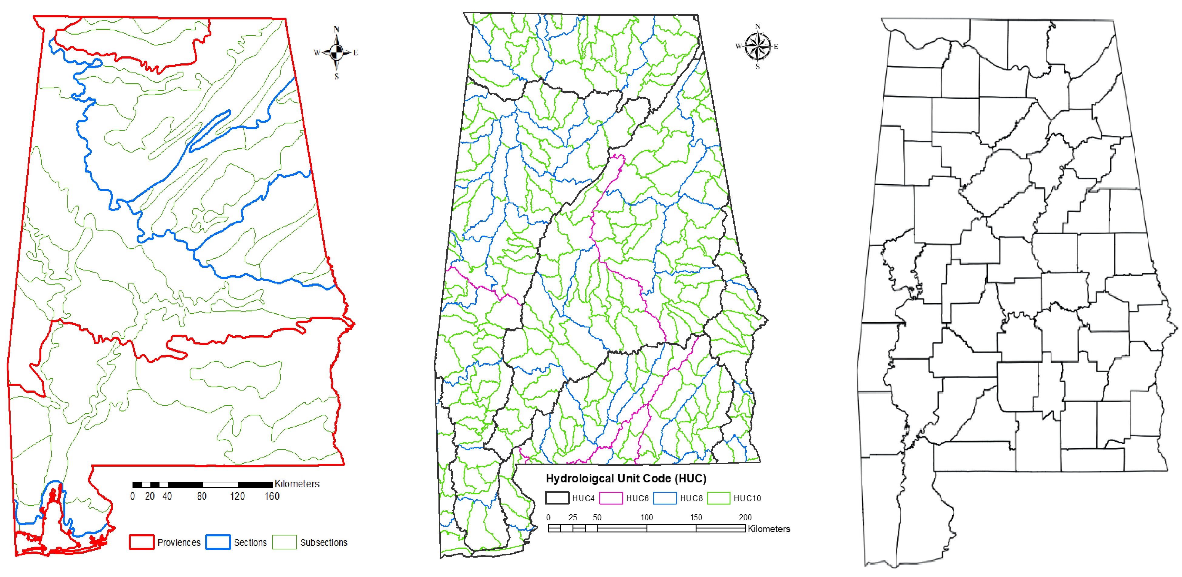
Figure 2.
Maps of spatial units (from coarse to fine): three levels of ecoregions (left), four levels of hydrological units (middle), and counties (right) used to predict the invasion of NNIPS in Alabama's forestlands.
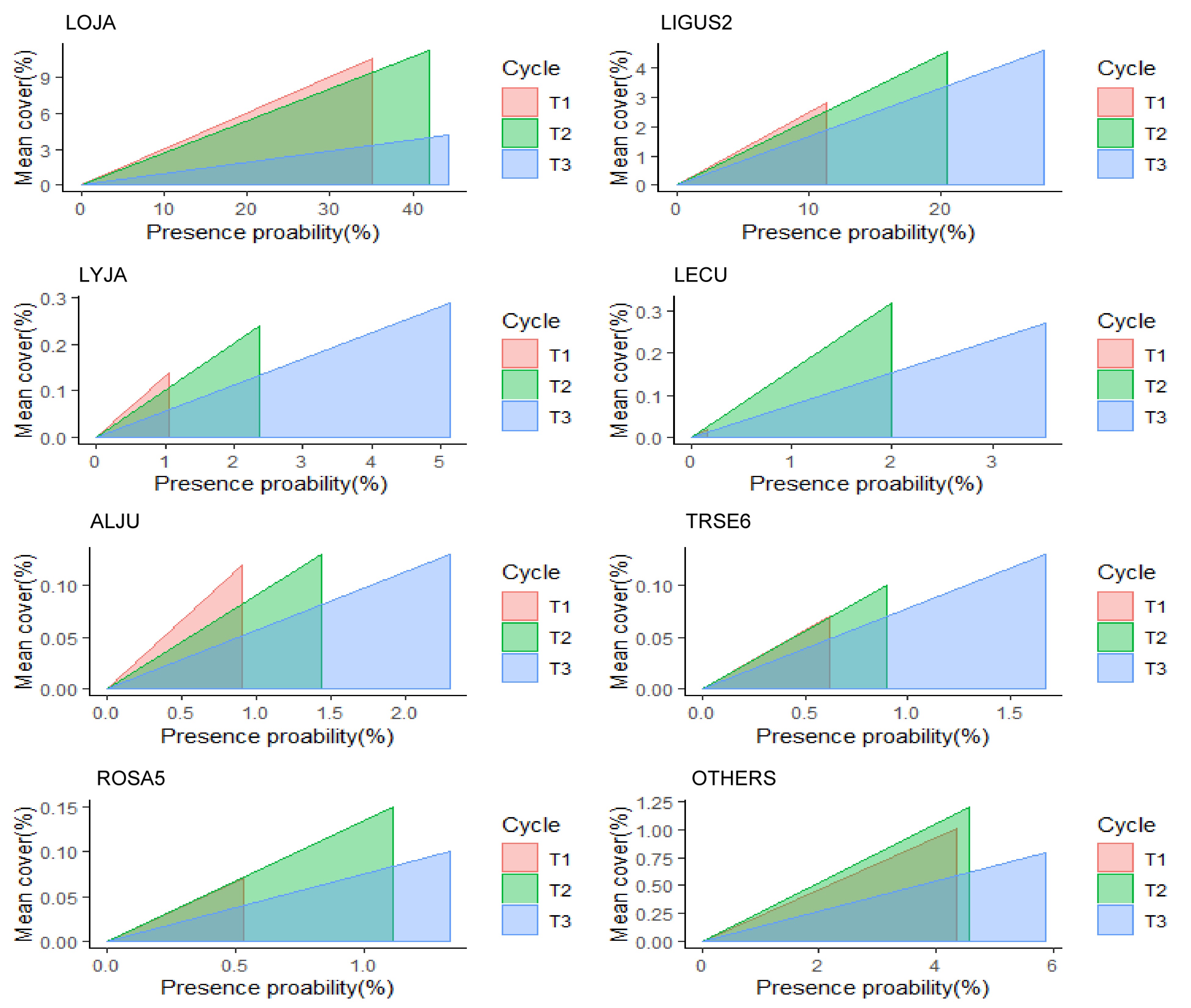
Figure 3.
Presence probability (x-axis) and mean cover percent (y-axis) of major NNIPS across all FIA subplots in Alabama's forestlands. NNIPS names in this figure based on FIA Vegetation Species Code (VEG SPCD); LOJA (Japanese honeysuckle), LIGUS2 (Privet), LYJA (Japanese climbing fern), LECU (Chinese lespedeza), ALJU (Silk-tree), TRSE6 (Chinese tallow tree), ROSA5 (Rose), and OTHERS (all other nonnative invasive plant species). The area inside triangles represents the invasion index (severity) and the shape of triangles represents whether an NNIP species is a fast-spreading species (larger changes in the presence probability) or a fast-establishing species (larger changes in the cover percentage) between different inventory cycles.
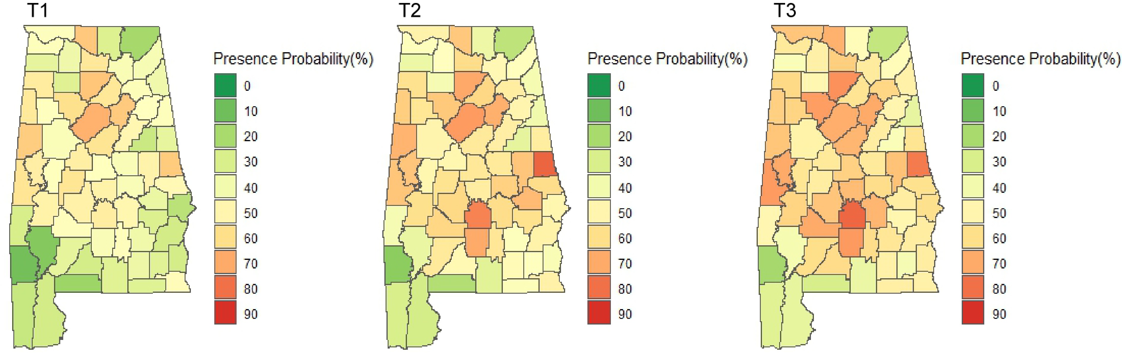
Figure 4.
Presence probability of all NNIPS in Alabama's forestlands over time (T1: 2001−2005, T2: 2006−2012, T3: 2013−2019).
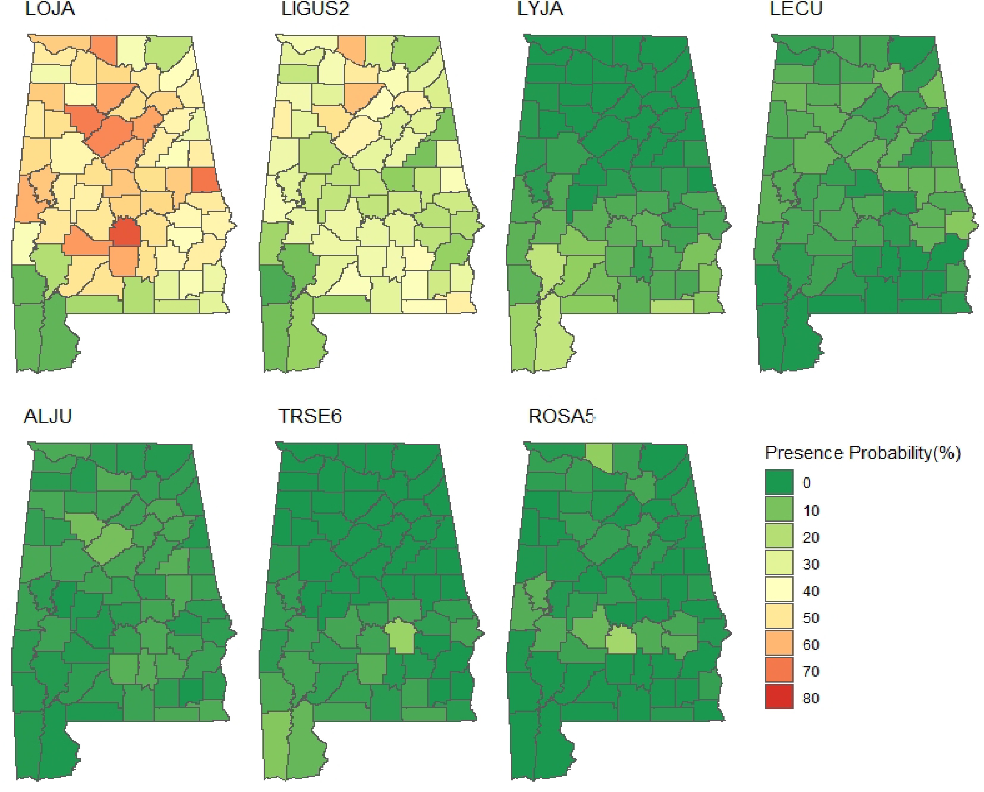
Figure 5.
Presence probability (%) of individual NNIPS measured between 2013 and 2019 in Alabama's forestlands. LOJA (Japanese honeysuckle), LIGUS2 (Privet), LYJA (Japanese climbing fern), LECU (Chinese lespedeza), ALJU (Silk-tree), TRSE6 (Chinese tallow tree), and ROSA5 (Rose).
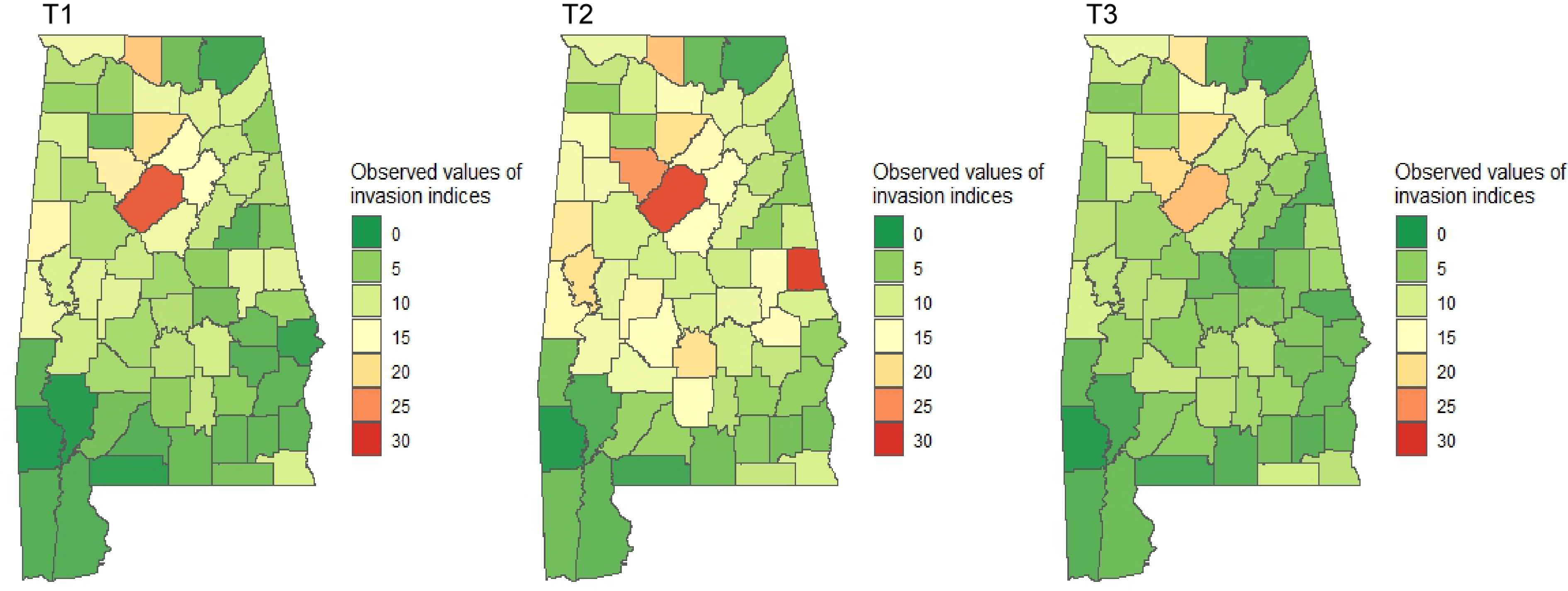
Figure 6.
Observed indices of invasion severity over time in Alabama's forestlands. Dark green represents the lowest and red represents the highest level of invasion.
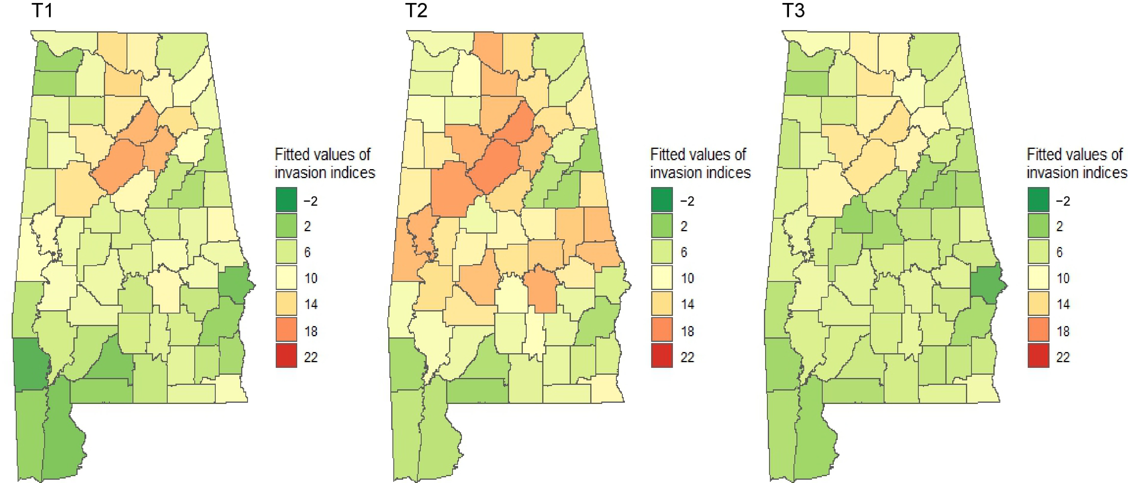
Figure 7.
Estimated indices of invasion severity by spatial lag models over time in Alabama's forestlands. Dark green represents the lowest and red represents the highest level of invasion.
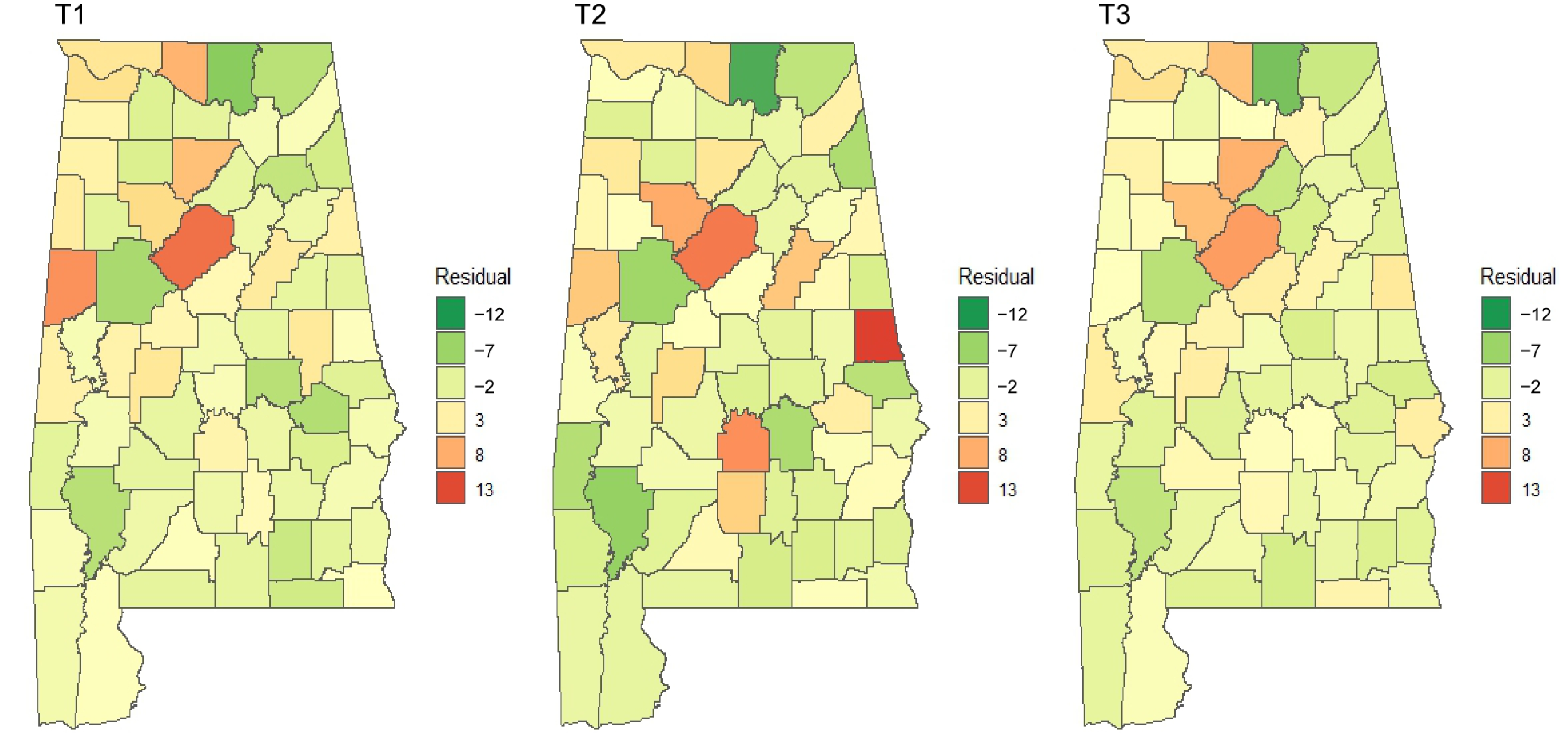
Figure 8.
Residuals of spatial lag models over time. The autocorrelation test of residuals is not statistically significant at the significance level of 0.05 (Table 5), which means the spatial lag models well fit the invasion patterns of NNIPS.

Variable	Variable definition	Data types	Data description and source
public_own_pct	Percent of publicly owned forest (0−100)	Ownership	FIA DataMart (https://apps.fs.usda.gov/fia/datamart/CSV/datamart_csv.html)
rd_length	Total length of major roads (interstate and state highways) (m)	Roads	Esri (www.arcgis.com/home/item.html?id=fc870766a3994111bce4a083413988e4)
rd_density	Road density in each county (m/m²)	Roads
elm_ash_cot	Elm/Ash/Cottonwood group area in percent (0−100)	Forest groups	USDA Forest Service (forest types/groups are based 2002 and 2003 data) https://data.fs.usda.gov/geodata/rastergateway/forest_type/index.php
lob_short	Loblolly/Shortleaf Pine group area in percent (0−100)
long_slash	Longleaf/Slash Pine group area in percent (0−100)
oak_gum_cypress	Oak/Gum/Cypress group area in percent (0−100)
oak_hickory	Oak/Hickory group area in percent (0−100)
oak_pine	Oak/Pine group area in percent (0−100)
lob	Loblolly Pine area in percent (0−100)	Forest types
lob_hard	Loblolly Pine/Hardwood area in percent (0−100)
long	Longleaf Pine area in percent (0−100)
mix_hard	Mixed Upland Hardwoods area in percent (0−100)
sw_no_wo	Sweetgum/Nuttall Oak/Willow Oak area in percent (0−100)
wo_ro_hi	White Oak/Red Oak/Hickory area in percent (0−100)
pop_2010	Population in 2010	Demographics	2010 US Census demographic information. Downloaded from Esri (https://hub.arcgis.com/datasets/esri::usa-counties/about)
pop_den_2010	Population density in 2010 (population·m²)
households	Number of households in 2010
pop_2010_nbh	Avg. population of neighborhood counties
pop_den_2010_ nbg	Avg. population density of neighborhood counties (population·m²)
ag_pct	Agriculture lands in percent (0−100)	Land-use	Land-use in 2016 from downloaded from LandFire (https://landfire.gov/viewer/viewer.html)
dev_pct	Developed lands in percent (0−100)
dist_pct	Disturbed lands in percent (0−100)
fr_pct	Forest lands in percent (0−100)
ot_pct	Other lands in percent (0−100)
wa_pct	Water cover in percent (0−100)
area	Total county area (m²)

Table 1.

Variables used in the spatial lag model to evaluate the potential driving factors of NNIPS invasions.

Measurement cycle	Year	Total subplots	Infested subplots	Infestation %	Invasive species count	Average species count per subplot (in infested subplots)
T1	2001−2005	15,240	6,268	41.1	8,251	1.32
T2	2006−2012	15,240	7,744	50.8	11,405	1.47
T3	2013−2019	15,240	8,347	54.8	14,020	1.68

Table 2.

Changes in the infestation rate (%) of NNIPS over time in Alabama's forestlands.

FIA species code	Common name	Latin name	Form	Infested subplot count			Presence probability (%)			Mean cover (%)
FIA species code	Common name	Latin name	Form	T1	T2	T3	T1	T2	T3	T1	T2	T3
LOJA	Japanese honeysuckle	Lonicera japonica Thunb	Vine	5,348	6,400	6,751	35.09	41.99	44.30	10.58	11.18	4.20
LIGUS2	Privet	Ligustrum L.	Shrub	1,740	3,122	4,248	11.42	20.49	27.87	2.80	4.55	4.59
LYJA	Japanese climbing fern	Lygodium japonicum (Thunb.)	Fern	162	360	781	1.06	2.36	5.12	0.14	0.24	0.29
LECU	Chinese lespedeza	Lespedeza cuneata (Dum. Cours.)	Forb	23	303	537	0.15	1.99	3.52	0.02	0.32	0.27
ALJU	Silk-tree	Albizia julibrissin Durazz.	Tree	139	219	351	0.91	1.44	2.30	0.12	0.13	0.13
TRSE6	Chinese tallow tree	Triadica sebifera (L.) Small	Tree	95	137	255	0.62	0.90	1.67	0.07	0.10	0.13
ROSA5	Rose	Rosa L.	Shrub	81	169	203	0.53	1.11	1.33	0.07	0.15	0.10
Others				663	695	894	4.35	4.56	5.87	1.01	1.21	0.80

Table 3.

Number of infested subplots by major NNIPS in Alabama's forestlands.

Modeling unit	T1			T2			T3
Modeling unit	Moran's I	Std error	p-value	Moran's I	Std error	p-value	Moran's I	Std error	p-value
HUC 4	−0.24	−0.32	0.63	0.02	0.09	0.18	−0.18	−0.08	0.53
HUC 6	0.14	1.36	0.09	0.32	2.38	0.01	0.18	1.64	0.05
HUC 8	0.27	3.19	< 0.001	0.35	3.98	< 0.001	0.23	2.68	< 0.001
HUC 10	0.36	10.49	< 0.001	0.36	10.36	< 0.001	0.26	7.35	< 0.001
HUC 12	0.24	15.08	< 0.001	0.18	11.59	< 0.001	0.18	11.29	< 0.001
COUNTY	0.40	5.55	< 0.001	0.38	2.25	< 0.001	0.37	5.23	< 0.001
Ecoregion (section)	0.37	2.14	0.02	0.51	2.44	0.01	0.27	2.00	0.02
Ecoregion (subsection)	0.06	0.82	0.21	0.01	0.37	0.35	0.01	0.28	0.39

Table 4.

Moran's I test of the invasion index of all NNIPS in Alabama's forestlands.

Measurement cycle (year)	Model statistics	Variable	Estimated coefficients	p-value	Residual autocorrelation
Measurement cycle (year)	Model statistics	Variable	Estimated coefficients	p-value	Test z-value	p-value
T1 (2001−2005)	lag coefficient ρ = 0.51 (p < 0.001) AIC = 390.5	intercept	4.681	0.085	0.551	0.458
		pop_2010_nbh	0.029	0.020
		rd_density	19.016	0.041
		oak_pine	−0.187	0.124
		lob_hard	−0.273	0.116
		mix_hard	−0.106	0.139
		wo_ro_hi	−0.172	0.027
		public_own_pct	−0.086	0.110
		ot_pct	−113.519	0.011
		wa_pct	−21.017	0.085
T2 (2006−2012)	lag coefficient ρ = 0.53 (p < 0.001) AIC = 407.37	intercept	10.264	< 0.001	0.904	0.341
		pop_2010_nbh	0.024	0.058
		oak_pine	−0.281	0.036
		wo_ro_hi	−0.209	0.019
		elm_ash_cot	1.008	0.090
		public_own_pct	−0.175	0.006
		ot_pct	−168.324	0.001
T3 (2013−2019)	lag coefficient ρ = 0.55 (p < 0.001) AIC = 367.95	intercept	6.171	< 0.001	0.228	0.633
		pop_2010_nbh	0.029	0.003
		lob_hard	−0.483	< 0.001
		wo_ro_hi	−0.161	0.018
		public_own_pct	−0.122	0.007
		ot_pct	−80.554	0.034
		wa_pct	−14.603	0.127

Table 5.

Estimated regression coefficients and summary statistics of the fitted spatial lag models.