-
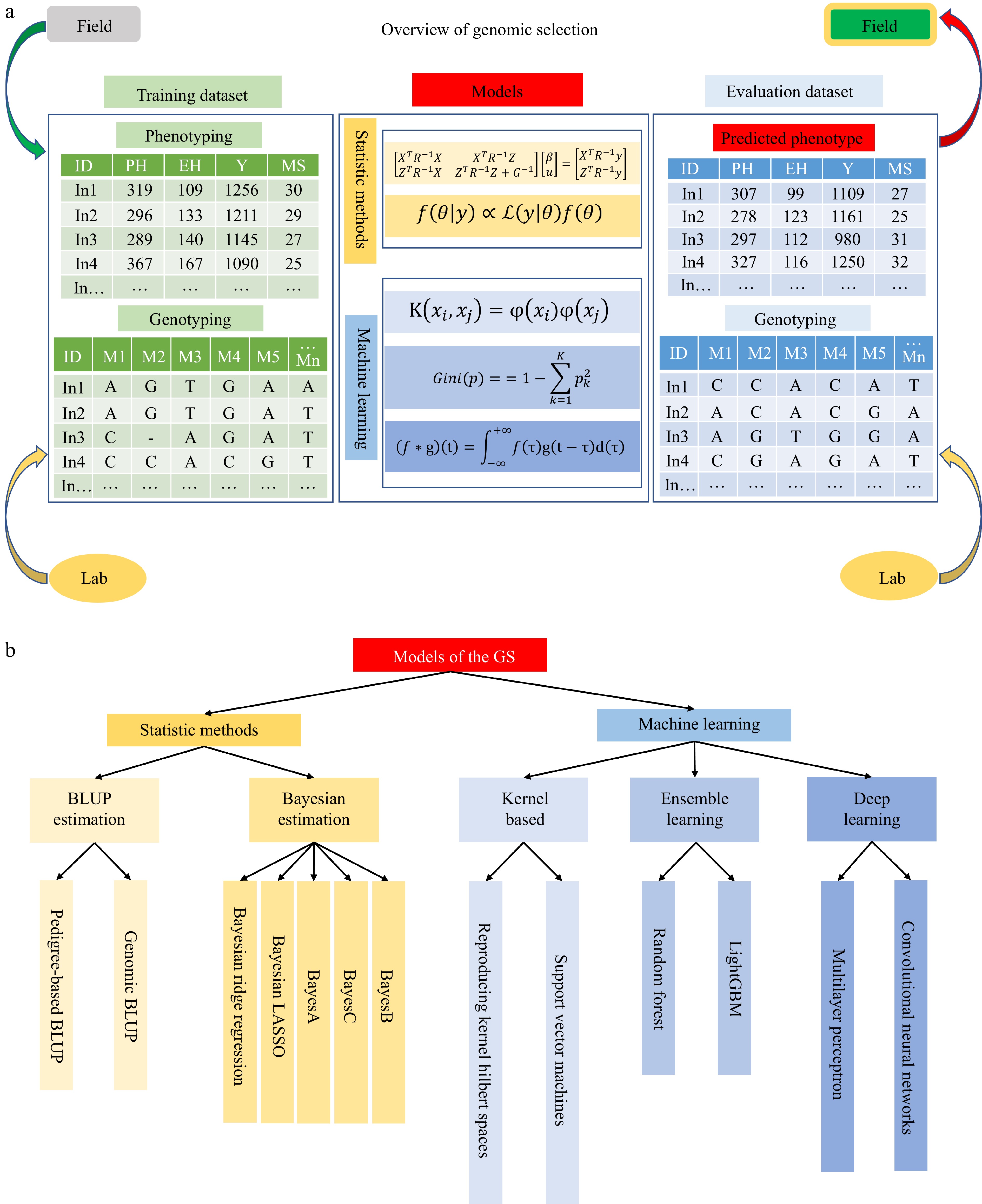
Figure 1.
An overview of genomic selection. (a) There are three parts in the genomic selection, including the training dataset, models, and evaluation dataset. The training dataset consists of phenotyping data collected from the field trials and genotyping data tested in the marker lab. The models are trained through two strategies: statistical methods and machine learning. The evaluation dataset is predicted phenotype and genotyping. The materials would be selected according to the predicted phenotyping and then go to field experiments. (b) Summary of models in GS.
-
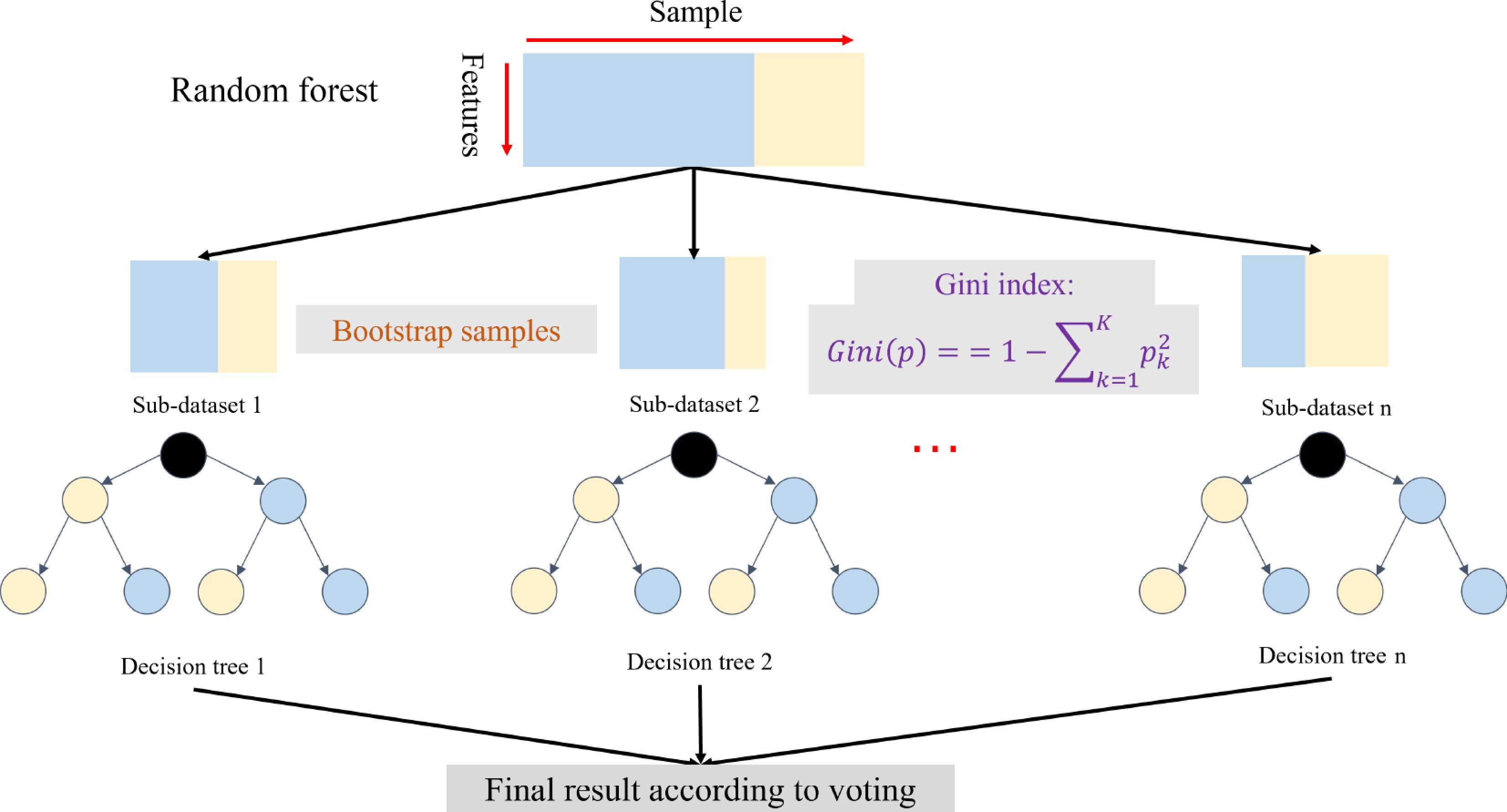
Figure 2.
An overview of the random forest[51]. The random forest includes the bootstrap samples and weak learners based on the decision tree with the Gini algorithm.
-
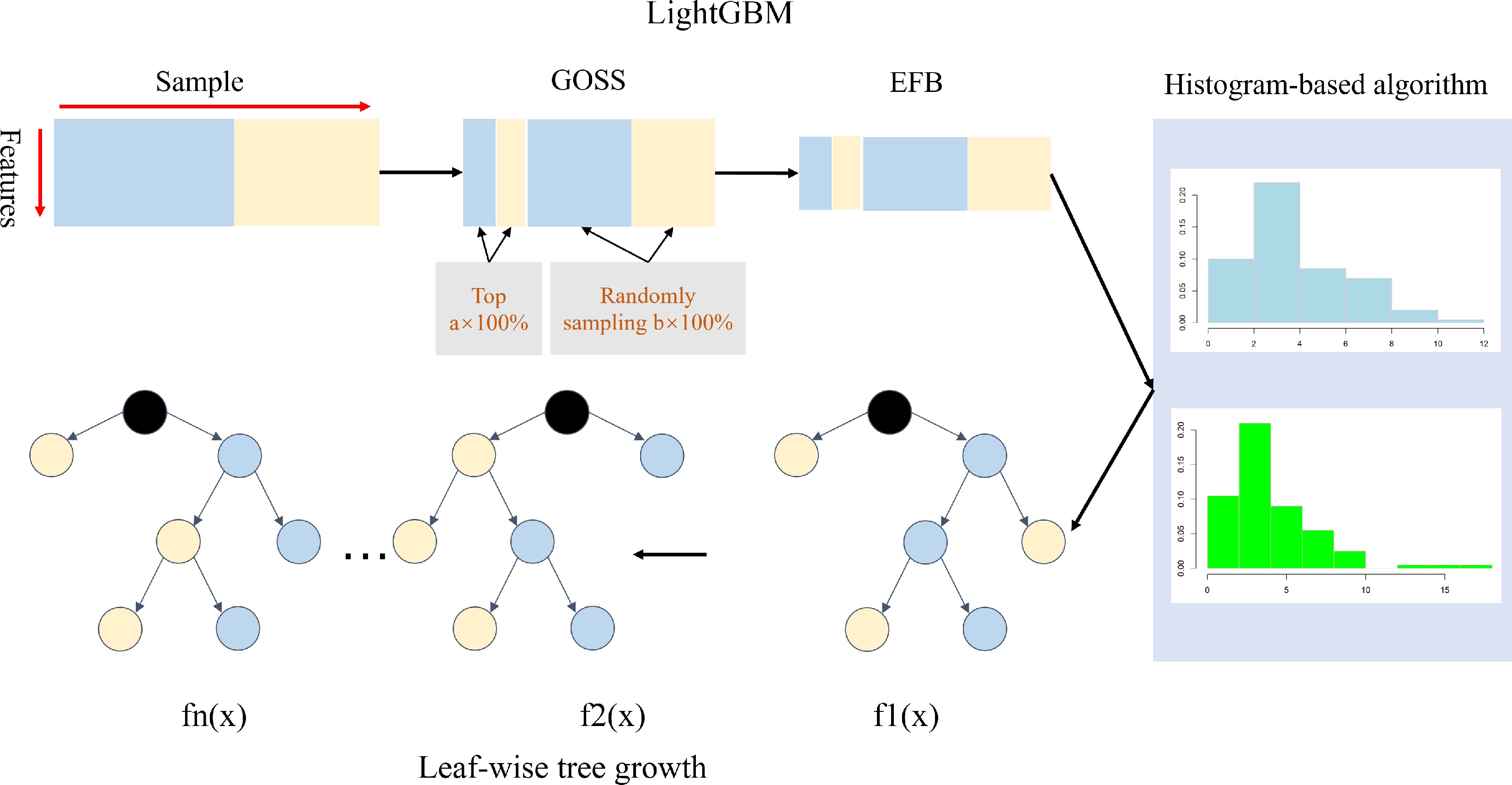
Figure 3.
An overview of LightGBM[57]. LightGBM includes the GOSS, EFB, histogram-based feature selection, and leaf-wise tree growth of the decision tree.
-
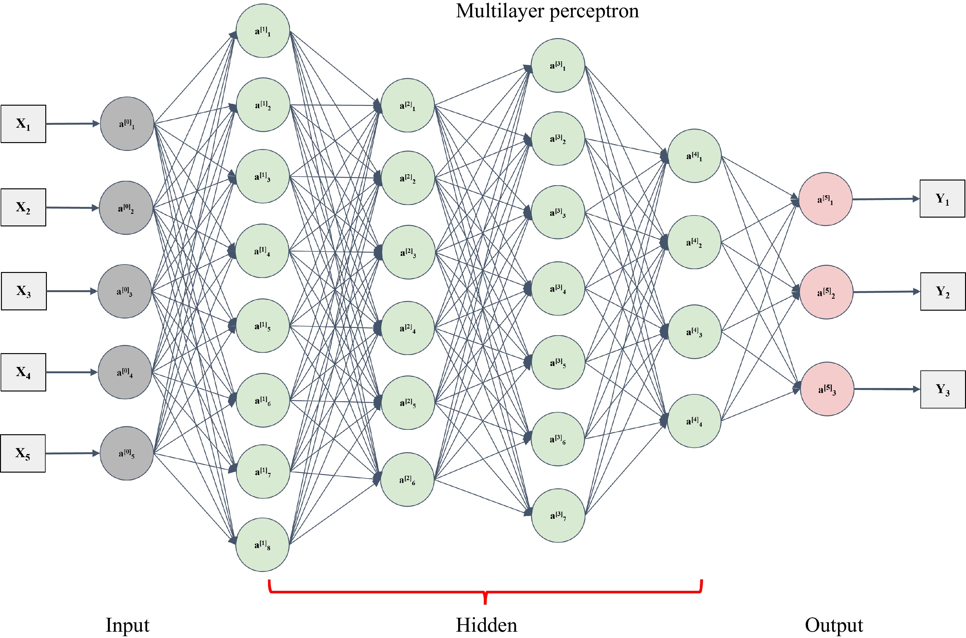
Figure 4.
An architecture of multilayer perceptron[62]. The multilayer perceptron includes one layer (a0 layer) with respect to input data and one layer (a5 layer) with respect to the output. The hidden layer could consist of many layers (from a1 to a4).
-
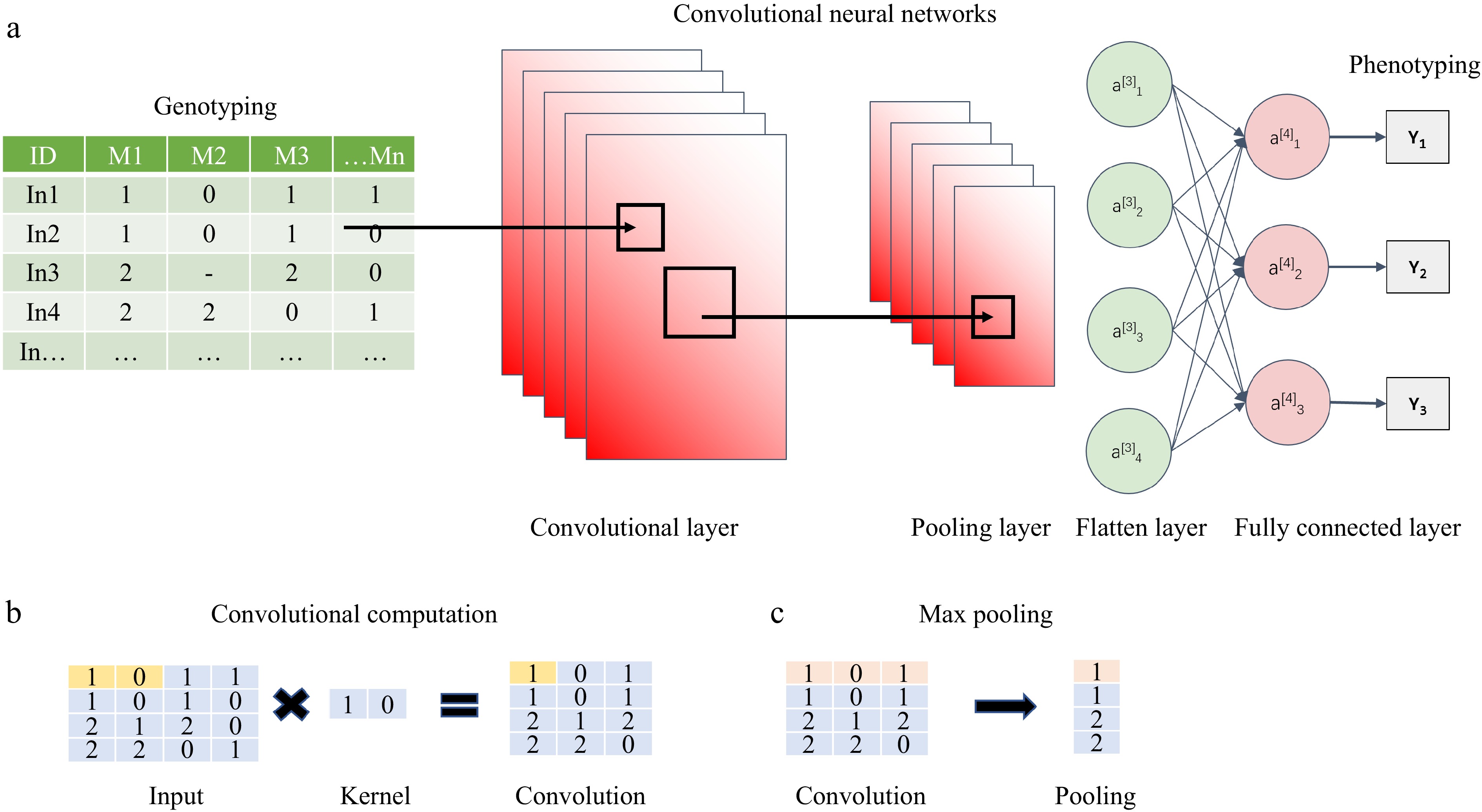
Figure 5.
An architecture of convolutional neural networks[67]. (a) General CNN algorithm, including convolutional layer, pooling layer, and fully connected layer. (b) Explanation of the convolutional computation. (c) Max pooling method.
-
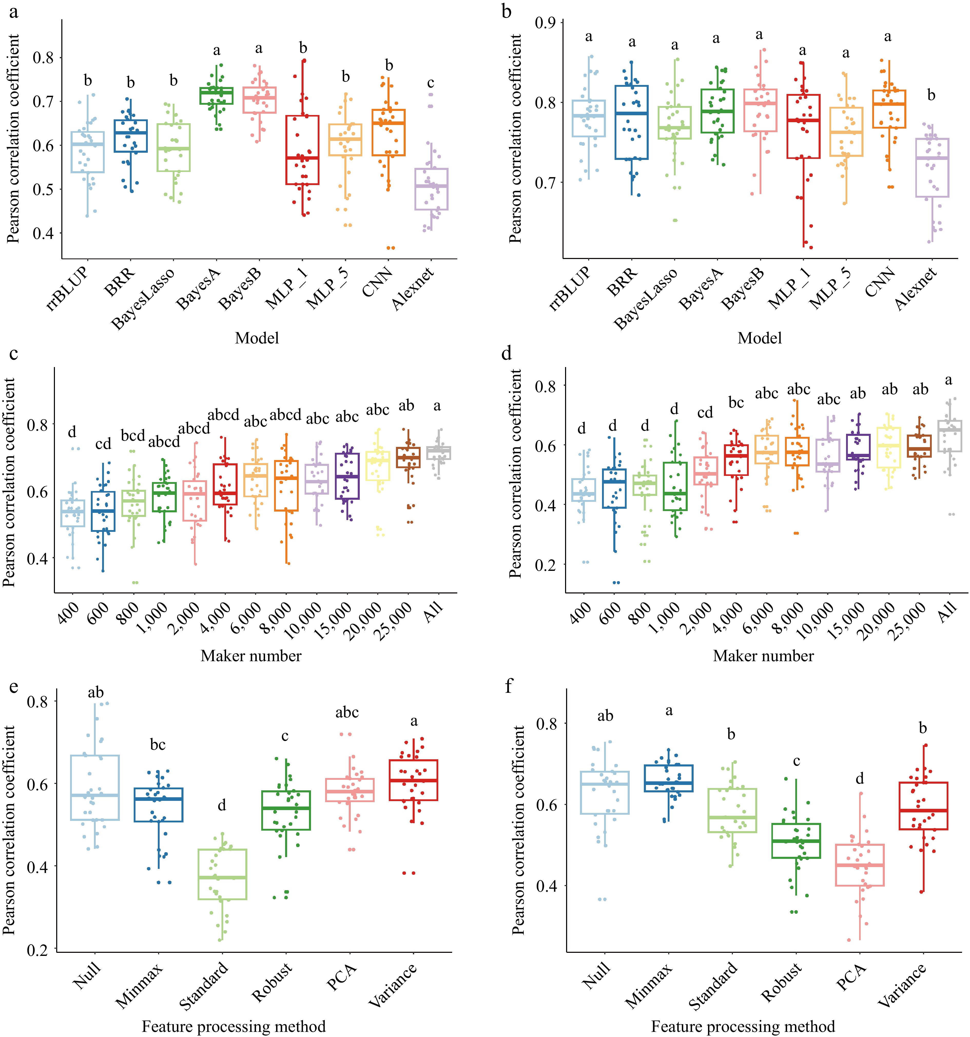
Figure 6.
Comparison of factors on GS models prediction ability. (a) and (b) comparison of nine GS algorithms on wheat based on the Pearson correlation coefficient of the model prediction ability. (a) Plant height with two major QTLs and heritability is 75.7% in 2014 and 76.5% in 2015, (b) yield with five major QTLs and heritability is 70.1% in 2014 and 85.6% in 2015. 'MLP_1' and 'MLP_5' denote the one and five hidden layers in multilayer perceptron algorithm; 'CNN' means the one convolutional layer, one pooling layer, one fully connected layer; 'Alexnet' is based on the Alexnet architecture model. (c) and (d) Impact of marker numbers on prediction accuracy. (c) Thirteen ways of markers set were randomly selected from 30548 markers to validate the prediction accuracy through the BayesA model. (d) Thirteen ways of markers set were randomly selected from 30548 markers to validate the prediction accuracy through the MLP_1 (multilayer perceptron algorithm with one hidden layer) model. (e) and (f) Impact of feature processing on prediction accuracy. (e) Six ways of feature processing were used to validate the prediction accuracy through the MLP_1 model. (f) Six ways of feature processing were used to validate the prediction accuracy through the CNN model. 'Null' is all markers; 'minmax' is min-max scaling; 'standard' is z-score normalization; 'robust' is robust feature processing; 'PCA' is principal component analysis; 'variance' is the variance scaling. Validation of all models is conducted by five-fold cross validation and repeat 30 times. The least significant difference (LSD) is used as the significance test with threshold of 0.05.
-
Comparison item ML-based GS algorithms Statistical algorithms Data handling capacity Process high-dimensional datasets, handle omics data Limited to traditional markers Non-linear relationship Capture non-linear relationships and enhance model performance Struggle with non-linear relationships Computational resources Require significant computational resources Require fewer resources Interpretability Act as black boxes, difficult to interpret Provide transparent models Applicability Offer flexible processing, require tuning Suit linear relationships Table 1.
Comparison of ML-based GS algorithms and statistical algorithms.
-
Crop Population size Marker no. Performance Ref. Wheat 2,374 39,758 GBLUP ≥ MLP [63] Wheat 250 12,083 GBLUP ≥ MLP [63] Wheat 693, 670, 807 15,744 GBLUP ≥ MLP [63] Maize 309 158,281 GBLUP ≥ MLP [63] Wheat 767, 775, 964,
980, 945, 1,1452,038 GBLUP ≥ MLP ≈ SVM [64] Maize 2,267 19,465 MLP > Lasso [100] Maize 4,328 564,692 GBLUP ≈ BayesR ≈ SVM [49] Barley 400 50,000 Transformer ≈ BLUP [83] Maize 8,652 32,559 LightGBM > rrBLUP [60] Wheat 2,000 33,709 LightGBM ≈ DNNGP > GBLUP [70] Maize 1,404 6,730,418 SVR ≈ DNNGP > GBLUP [70] Wheat 599 1,447 SVR ≈ DNNGP > GBLUP [70] Table 2.
Summary of the performance between the ML and traditional methods.
Figures
(6)
Tables
(2)