-
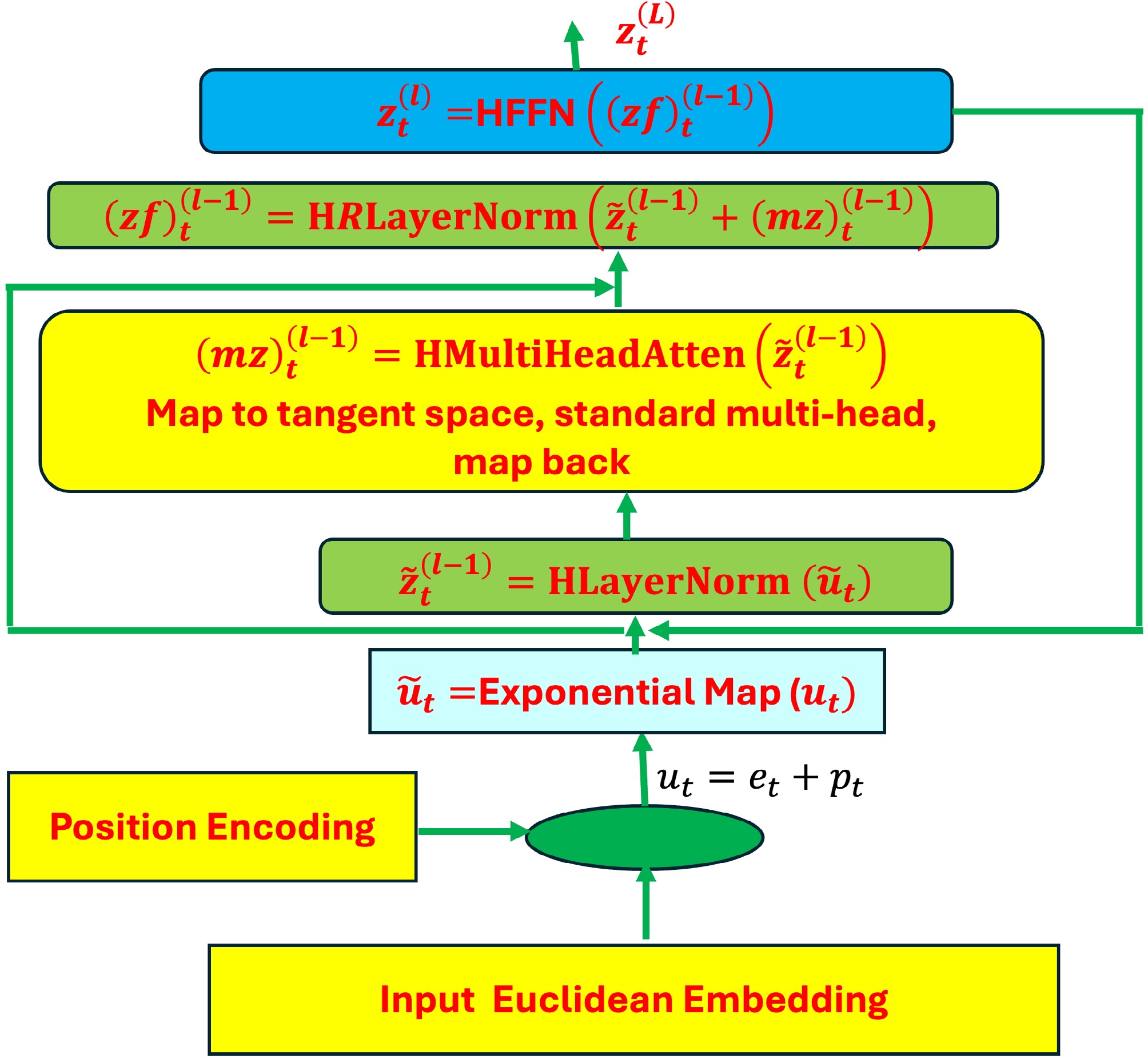
Figure 1.
Architecture of hyperbolic transformers. All steps: input Euclidean embedding, position encoding, hyperbolic layer normalization, hyperbolic multi-head attention, and hyperbolic feed-forward neural networks in the hyperbolic transformer encoder block.
-

Figure 2.
Transition function learning. A hyperbolic transformer is employed to learn the dynamics of the environment by modeling the transition function in RL, which describes how the environment transitions from the current state s to the next state s' and issues rewards r in response to the actions taken by the agent.
-
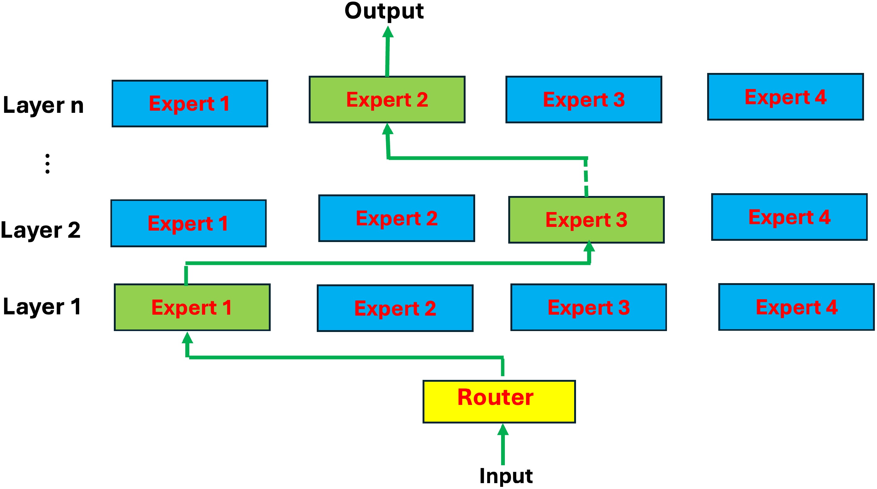
Figure 3.
Outline of MoE. The MoE has two main components, namely experts and the router: experts − each FNN layer now has a set of 'experts' which are subsets in the FNN. Router or gate network − the router determines how input tokens’ information passes experts. The MoE replaces FFN in the transformer.
-
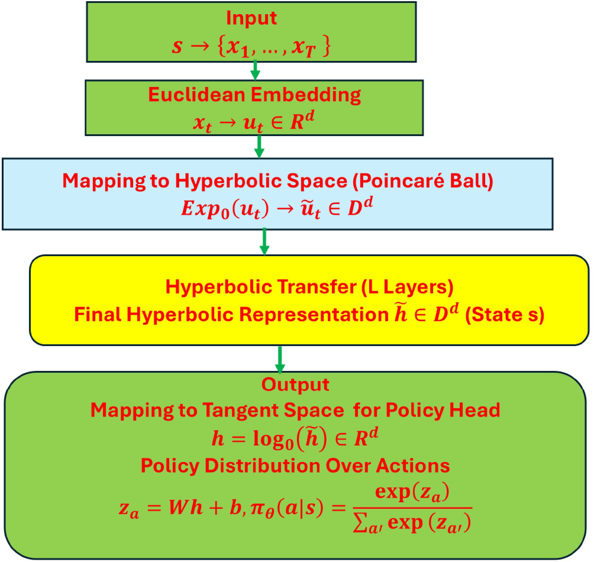
Figure 4.
Hyperbolic transformer as a policy.
-
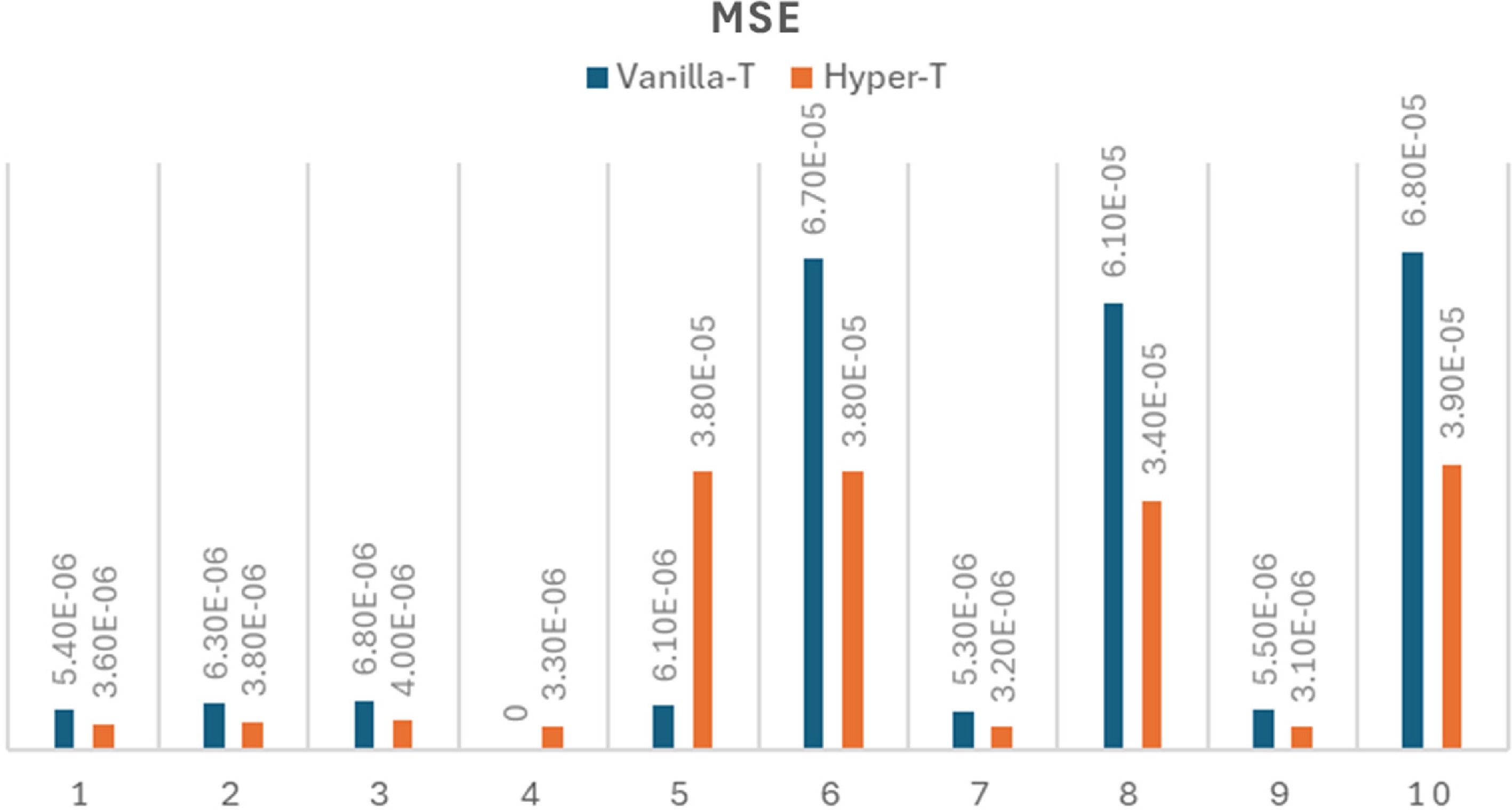
Figure 5.
MSE of vanilla-transformer and hyperbolic-transformer for solving ten FrontierMath problems (excluding A.11 sample problem 11 - prime field continuous extensions).
-
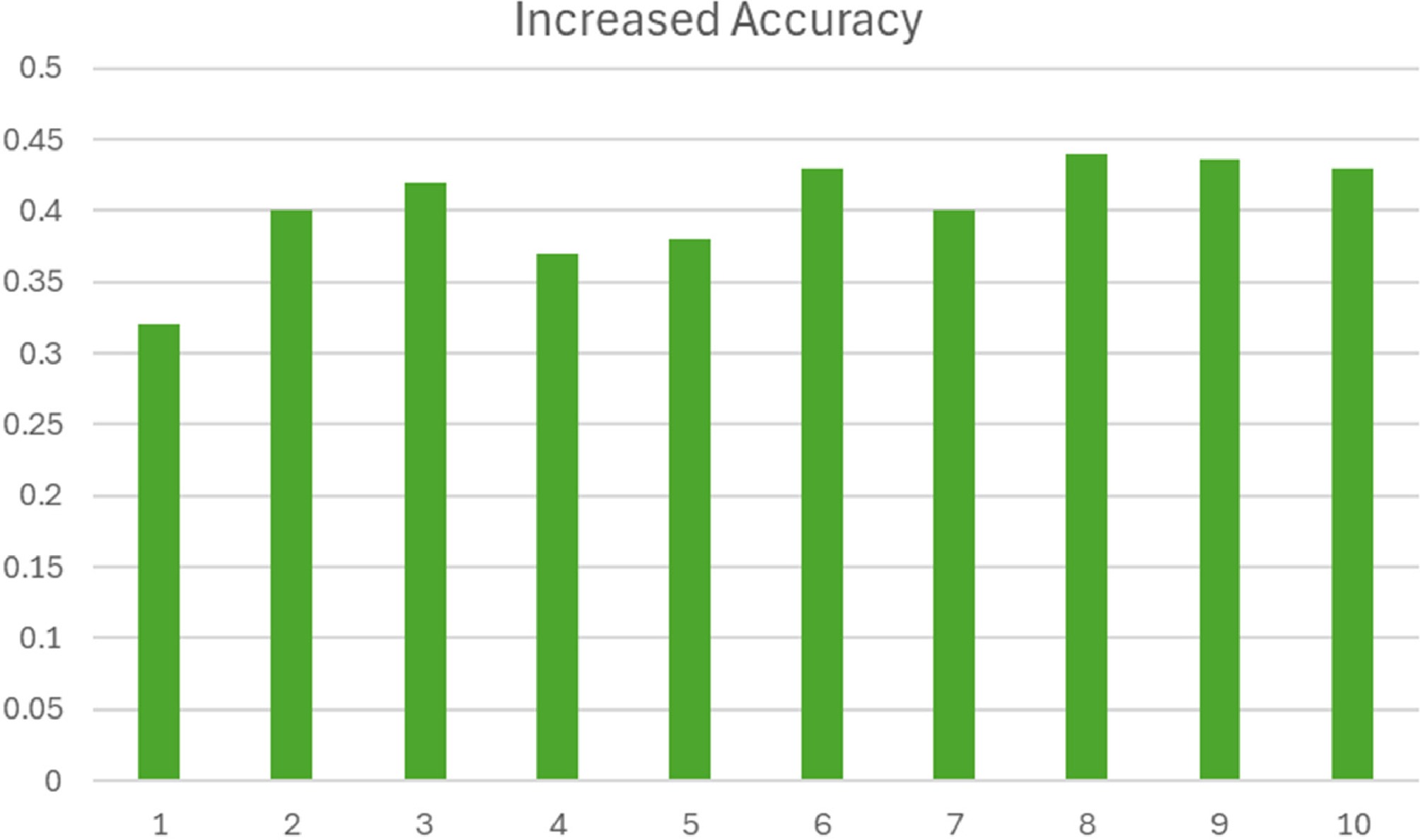
Figure 6.
The increased accuracy of the Hyper-T vs Vanilla-T.
-

Figure 7.
Wall-ClockHyper-T for 11 FrontierMath problems.
-
Input: θ0: hyperbolic transformer, Manifold: the Poincaré ball, group G, clip ε Initialize policy πθ and hyperbolic transformer for k = 0, 1, 2, ... for env episode e = 1, ..., B 1. Sample collection from the policy A batch of N states $ {\{{s}^{\left(j\right)}\}}_{j=1}^{N} $ $ {\pi }_{{\theta }_{k}} $ For each state s(j), generate G responses: a set (or group) of G actions is sampled: $ \left\{{a}_{1}^{\left\{j\right\}}, \dots ,{a}_{G}^{\left\{j\right\}}\right\} $ $ r\left({s}^{\left(j\right)},{a}^{\left(j\right)}\right) $ With batch 2. Compute group-based (relative) advantage Define the group statistics for each state s(j) and its corresponding group of actions, then, defining the group-relative advantage for each action $ {a}_{i}^{\left(j\right)} $ $ \left({s}^{\left(j\right)},{a}_{i}^{\left(j\right)}\right) $ $ {\pi }_{{\theta }_{k}}\left({a}_{i}^{\left(j\right)}|{s}^{\left(j\right)}\right) $ $ {D}_{KL}\left({\pi }_{{\theta }_{k}}\left|\right|{\pi }_{ref}\right) $ 3. Form the GRPO surrogate objective $ L\left({s}^{\left(j\right)},{\theta }_{k}\right) $ $ L\left({\theta }_{k}\right)=\dfrac{1}{N}{\sum }_{j=1}^{N}L\left({s}^{\left(j\right)},{\theta }_{k}\right). $ End batch 4. Gradient ascent through hyperbolic transformations and hyperbolic-aware optimization for updating parameters. End k Table 1.
hyperbolic GRPO.
-
Backbone Updates to MAE < 10−6 Final MAE × 10−6 Wall-clock Vanilla-T 10,200 ± 800 6.2 1 Hyperbolic-T 6,600 ± 610 3.1 0.84 × Table 1.
Comparison between vanilla transformer and hyperbolic transformer on the scalar root-finding benchmark.
-
Backbone Updates to hit 11 Miss.pred.rate (%) Wall-clock Vanilla-T 10,400 ± 800 0.46 1.00 Hyper-T 6,900 ± 600 0.31 0.83 Table 2.
Comparison between vanilla transformers and hyperbolic transformers on the Prime field continuous extension problem.
-
Backbone Updates to MAE < 10−6 Final MAE × 10−6 Wall-clock Vanilla-T 12,800 ± 900 6.4 1.00 Hyper-T 8,200 ± 670 3.6 0.83 Table 3.
Comparison between vanilla transformer and hyperbolic transformers on the Van-der-Pol optimal-control problem.
-
Backbone Updates to MAE < 10−6 Final MAE ×10−6 Wall-clock Vanilla-T 10,500 ± 800 6.0 1.00 Hyper-T 6,800 ± 620 3.3 0.84 Table 4.
Comparison between vanilla transformer and hyperbolic transformers on the unicycle–vehicle energy-minimization problem.
Figures
(7)
Tables
(5)