-
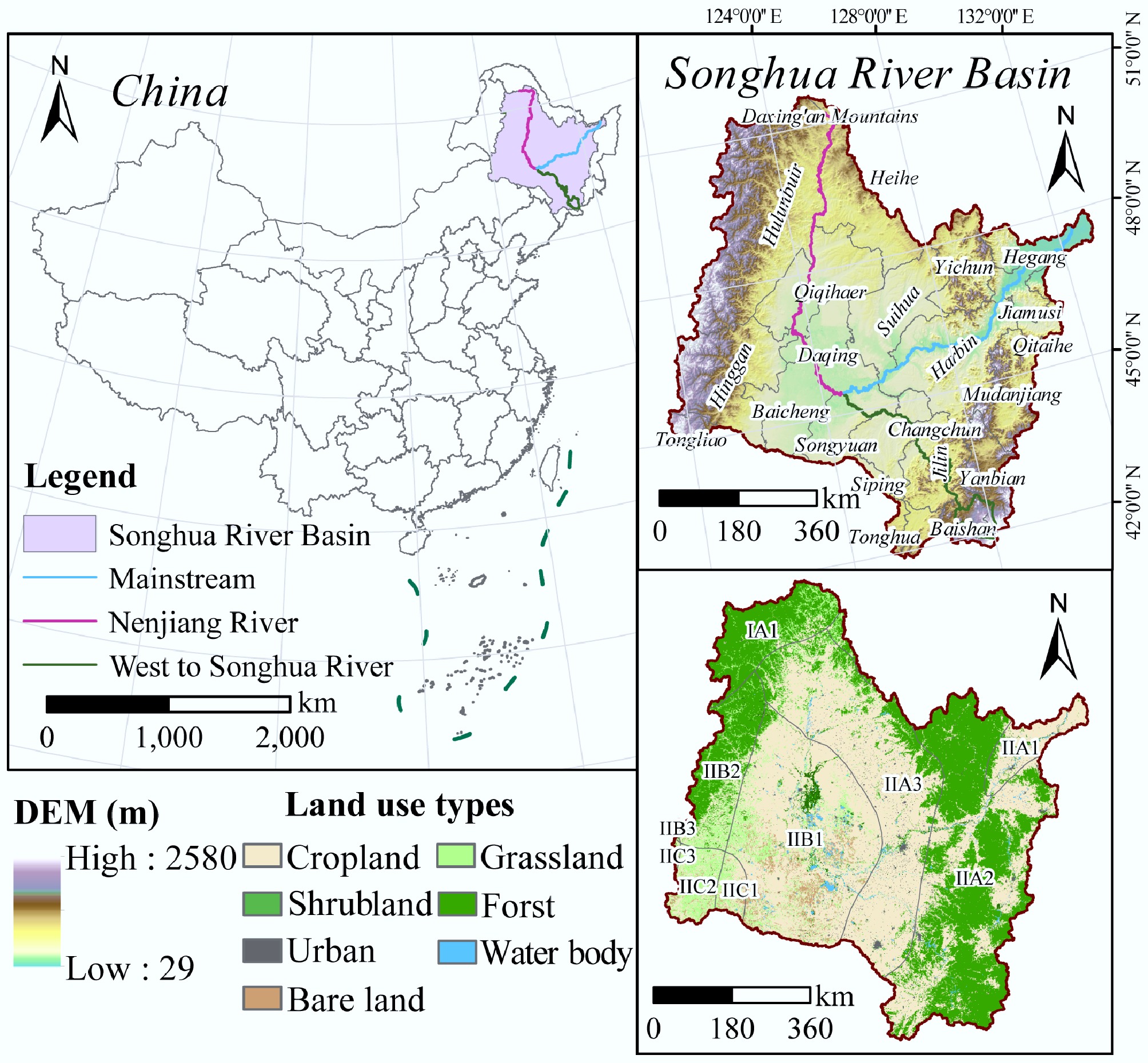
Figure 1.
Geographical location and land use types in the SRB. The basin is divided into ten eco-geographical sub-regions: IA1 (Greater Khingan Mountains), IIA1 (Sanjiang Plain), IIA2 (Eastern Uplands of Northeast China), IIA3 (Front Mountain Plain of Eastern Northeast China), IIB1 (Central Songliao Plain), IIB2 (Southern Greater Khingan Mountains), IIB3 (Plain and Hills Sanhe Piedmont), IIC1 (Southwestern Songliao Plain), IIC2 (Northern Greater Khingan Mountains), and IIC3 (Eastern Inner Mongolia Plateau).
-
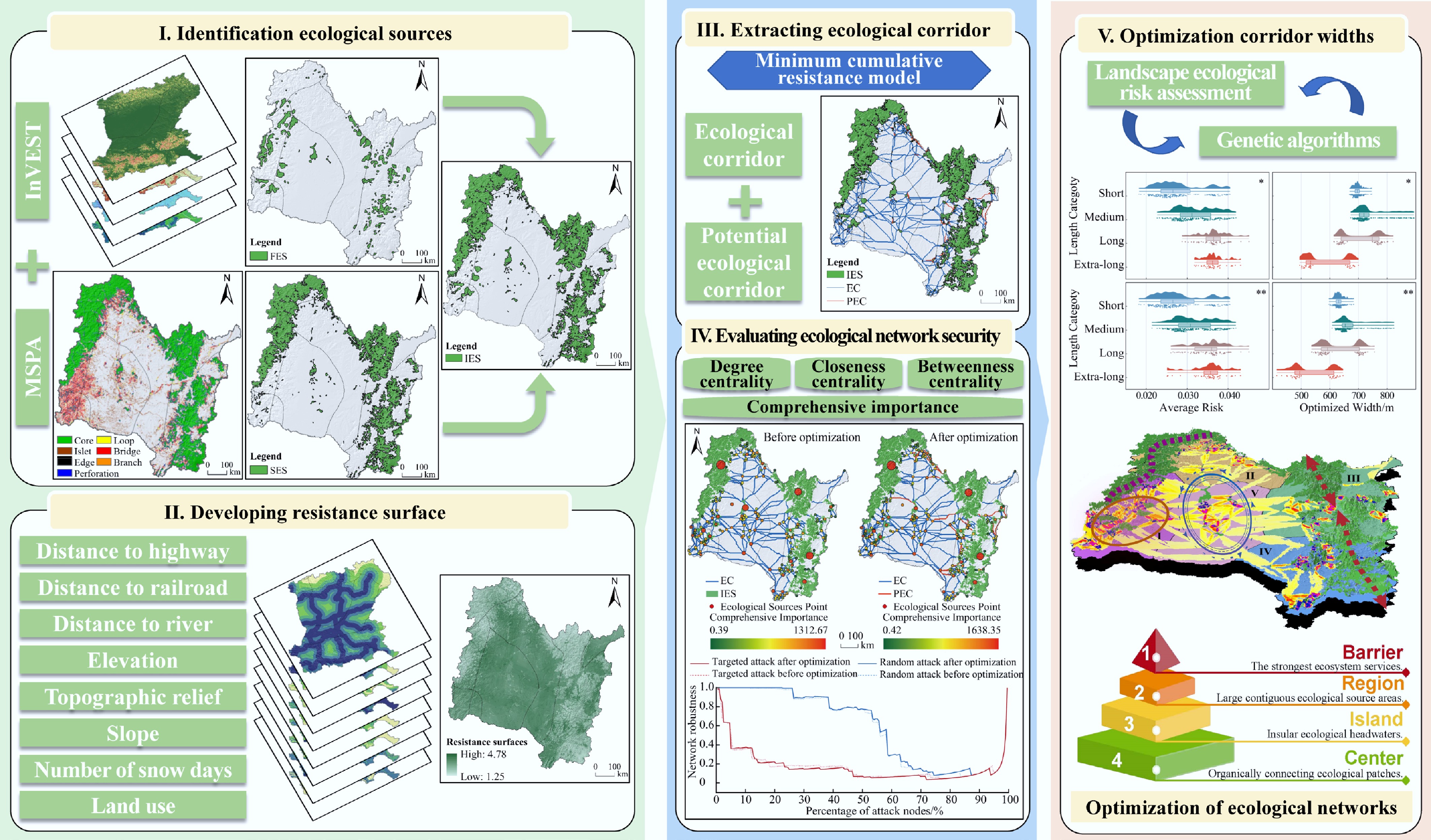
Figure 2.
The analysis framework of the study.
-
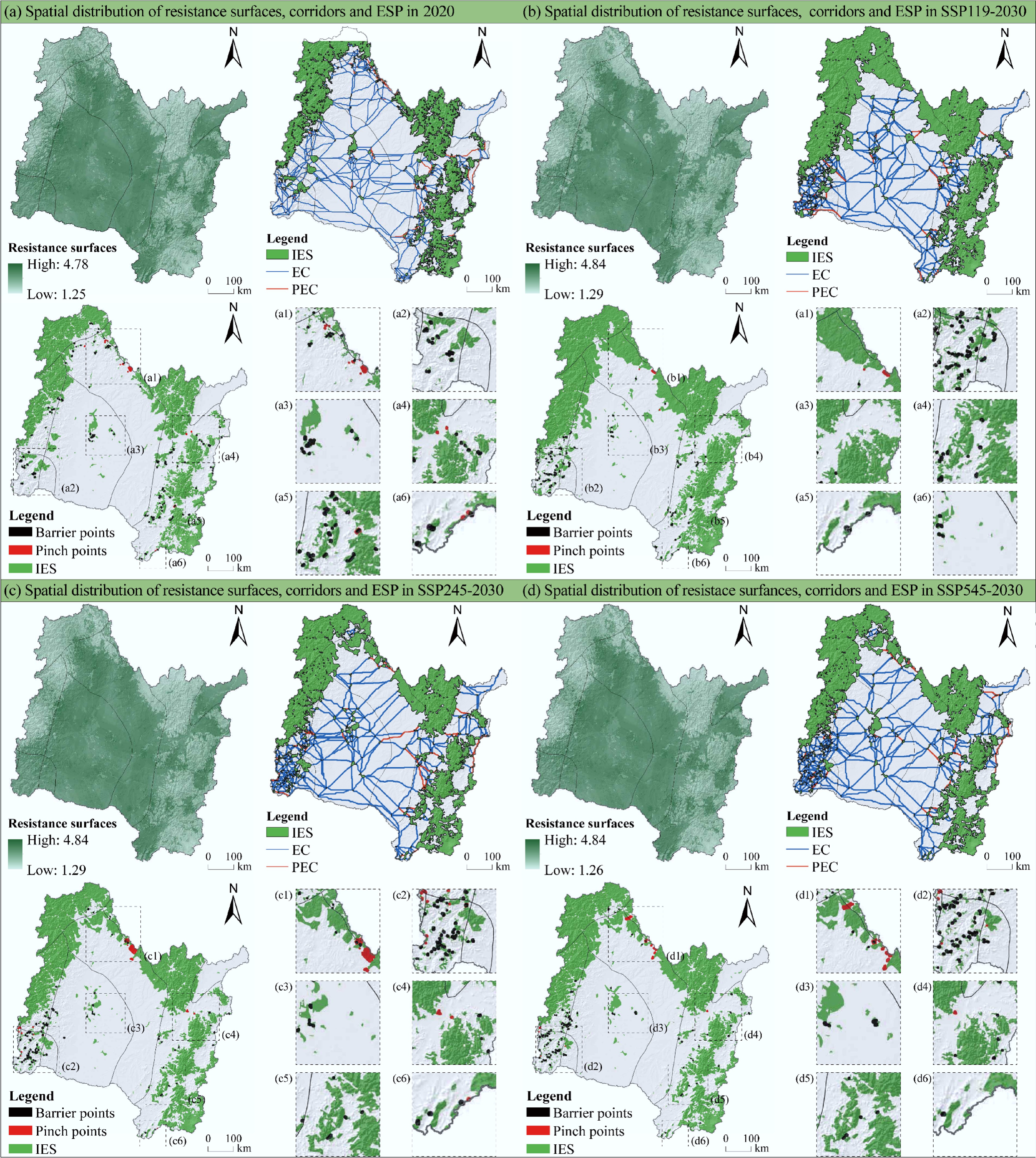
Figure 3.
Spatial distribution of resistance surfaces, corridors and the ESPs in the SRB. Panels (a)–(d) represent the years 2020, SSP119-2030, SSP245-2030, and SSP545-2030, respectively. ECs and PECs were identified using resistance surface methodology, and the specific locations of ecological pinch points and barrier points were analyzed. Panels (1)–(6) provide an enlarged view of these critical ecological pinch points and barrier points.
-
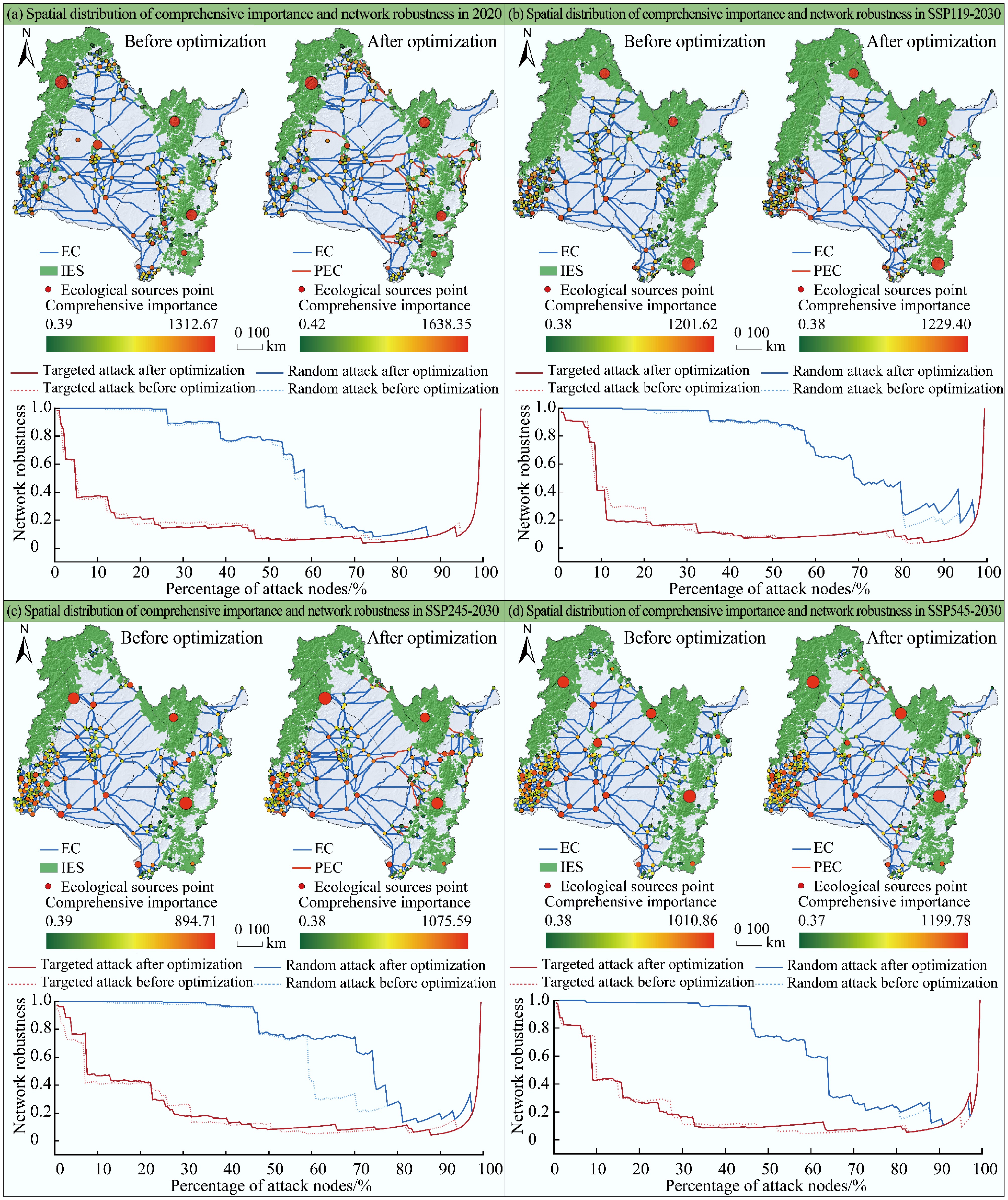
Figure 4.
Spatial distribution of CI and ecological network robustness in the SRB. Panels (a)–(d) represent the years 2020, SSP119-2030, SSP245-2030, and SSP545-2030, respectively. The figure compares overall importance metrics before and after optimization and evaluates the robustness of the ecological security network under both intentional and random attacks in the before and after optimization scenarios.
-
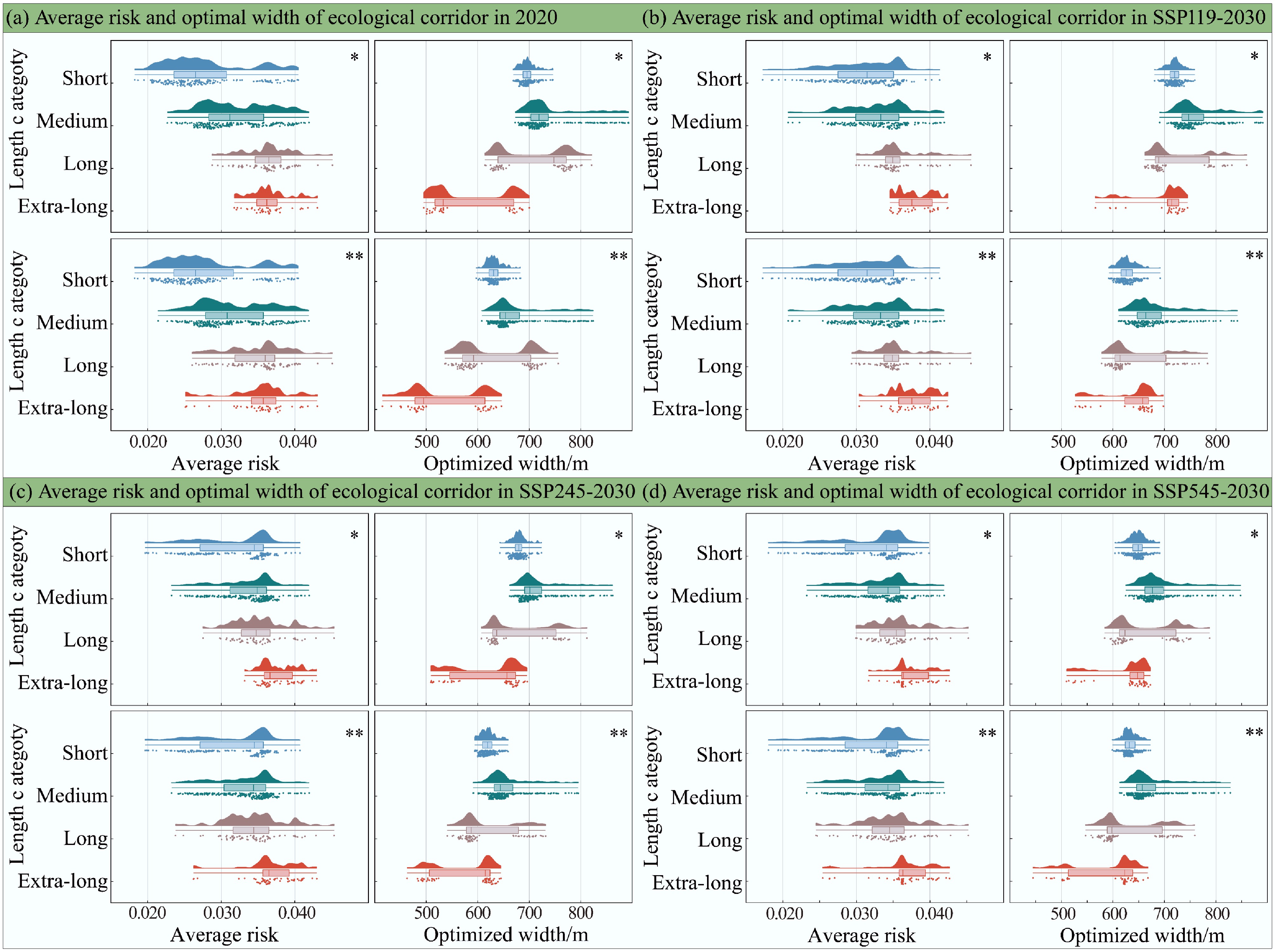
Figure 5.
Average risk and optimal width of ecological corridors in the SRB. Panels (a)–(d) represent the years 2020, SSP119-2030, SSP245-2030, and SSP545-2030, respectively. The figure compares the distribution of average risk and optimal corridor width both before (*) and after optimization (**).
-
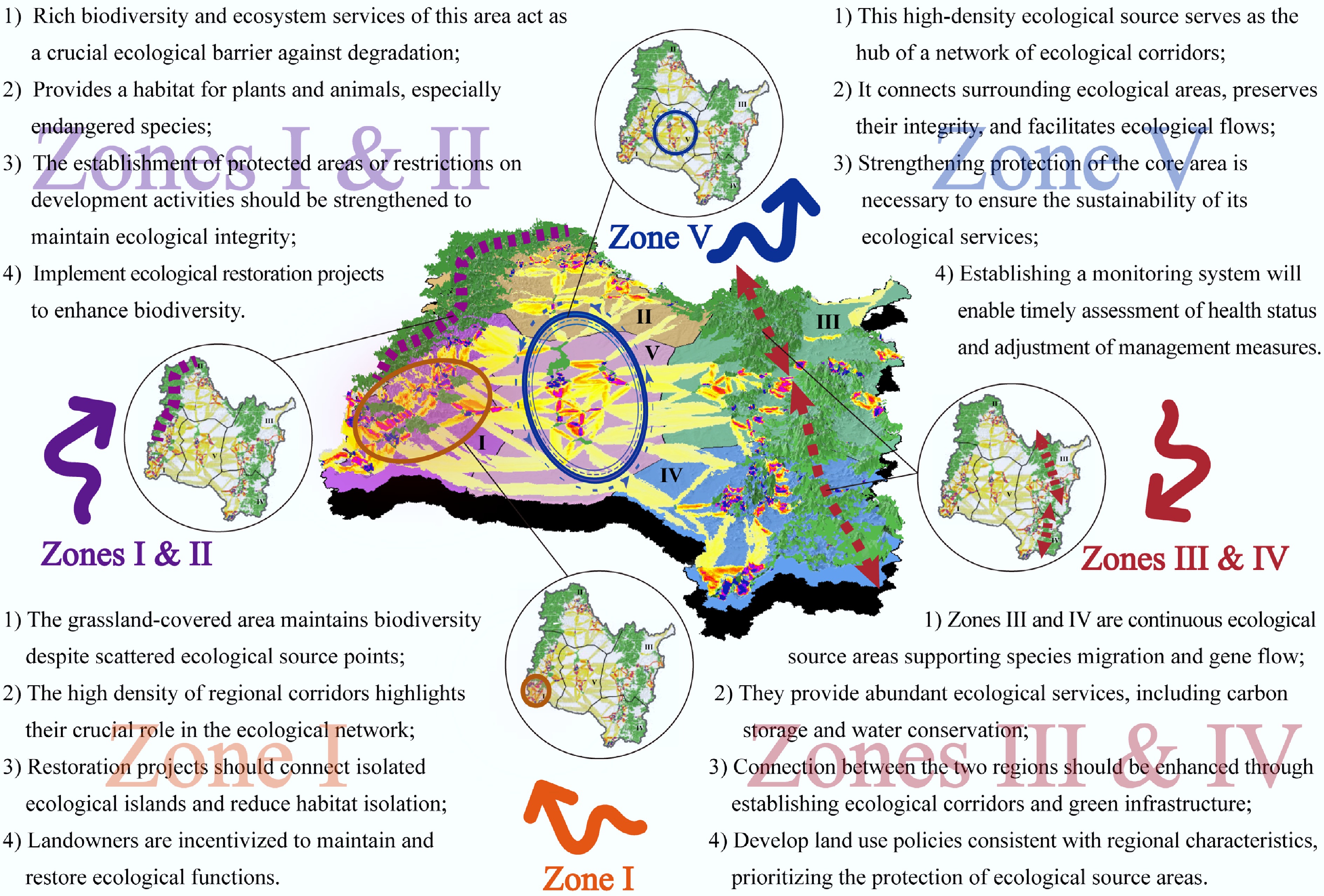
Figure 6.
Ecological security optimization patterns in the SRB. An ecological security barrier, referred to as the 'One barrier', was established between zones I and II. Two ecological source regions, termed the 'Two regions', were identified in zones III and IV, respectively. Numerous fragmented ecological source islands, designated as the 'Multiple islands', were observed in zone I. In the center of zone V, a dense ecological source with high current density was identified, forming the intersection center of ECs, referred to as the 'One center'.
-
Data Data sources Data description Land use data in 2020 Global ESA CCI land cover classification map ( http://maps.elie.ucl.ac.be/CCI/viewer )Raster, 300 m × 300 m Future scenario land use data in 2030
(SSP119, SSP245, and SSP545)Scientific Data[39] Raster, 1,000 m × 1,000 m Digital evaluation model (DEM) Geospatial Data Cloud (China) ( www.gscloud.cn )Raster, 30 m × 30 m Net primary productivity (NPP) United States Geological Survey (USGS) website ( https://lpdaac.usgs.gov/product_search/?view=list )Raster, 500 m × 500 m Soil profile Harmonized World Soil Database (HWSD v1.2) ( www.fao.org/soils-portal/data-hub/soil-maps-and-databases/harmonized-world-soil-database-v12 )Raster, 1,000 m × 1,000 m Road networks and river data China National Catalogue Service for Geographic Information ( www.webmap.cn )Vector Depth to bedrock map Scientific Data[40] Raster, 1,000 m × 1,000 m Eco-geographical region data Resource and Environment Science and Data Center ( www.resdc.cn/data.aspx?DATAID=125 )Vector Snow cover days (SCD) Earth System Science Data[41] Raster, 5,000 m × 5,000 m Table 1.
Data sources and description
-
Index name Computing formula Parameter description Landscape disturbance index (Di) $ {D_i} = a{F_i} + b{S_i} + c{E_i} $ (2) Weights: a = 0.5, b = 0.3, c = 0.2 Landscape fragmentation index (Fi) $ {F_i} = \dfrac{{{n_i}}}{{{A_i}}} $ (3) ni: patch count of the land use type i; Ai: total area of land use type i Landscape separation index (Si) $ {S_i} = \dfrac{A}{{2{A_i}}}\sqrt {\dfrac{{{n_i}}}{{{A_i}}}} $ (4) Where, ni is the patch count of the A: total area of the study region Landscape fractal dimension index (Ei) $ {E_i} = \dfrac{{2\ln \left(\dfrac{{{p_i}}}{4}\right)}}{{\ln ({A_i})}} $ (5) pi: proportion of patch count of land use type i to total patch count Table 2.
Landscape pattern indices and their significance
-
Indicator 2020 SSP119-2030 SSP245-2030 SSP545-2030 EC EC + PEC EC EC + PEC EC EC + PEC EC EC + PEC DC 5.08 5.68 5.29 5.58 5.21 5.66 5.30 5.65 CC 0.23 0.26 0.23 0.24 0.21 0.23 0.21 0.22 BC 189.92 189.32 171.71 171.42 190.79 190.34 203.70 203.35 CI 56.59 56.41 48.04 48.09 53.37 52.43 57.66 56.13 Table 3.
Mean values of the ecological network topology indicators
Figures
(6)
Tables
(3)