-
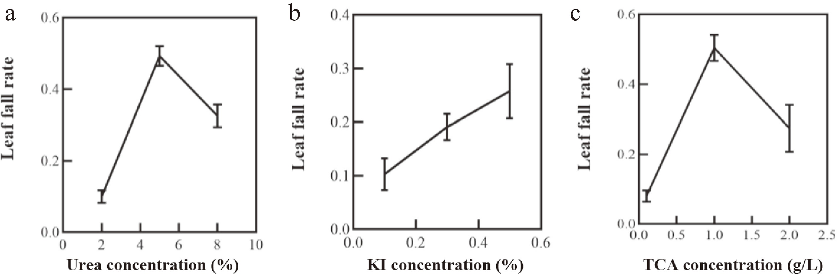
Figure 1.
The effects of (a) urea, (b) potassium iodide (KI), and (c) trichloroacetic acid (TCA) concentrations on the leaf fall rate of apples.
-
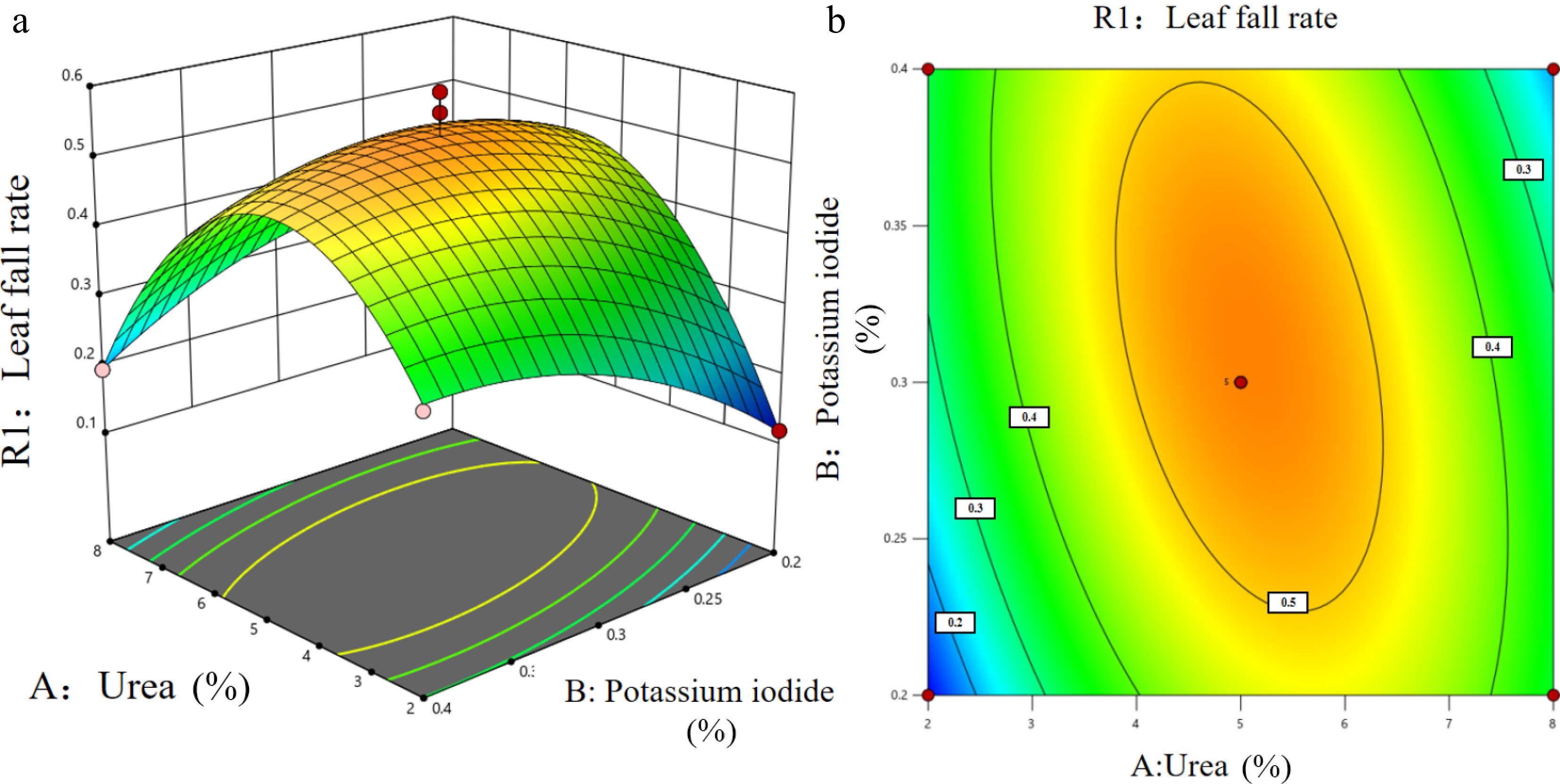
Figure 2.
Response surface diagram of interaction to (a) apple leaf fall rate, and (b) contour plot.
-
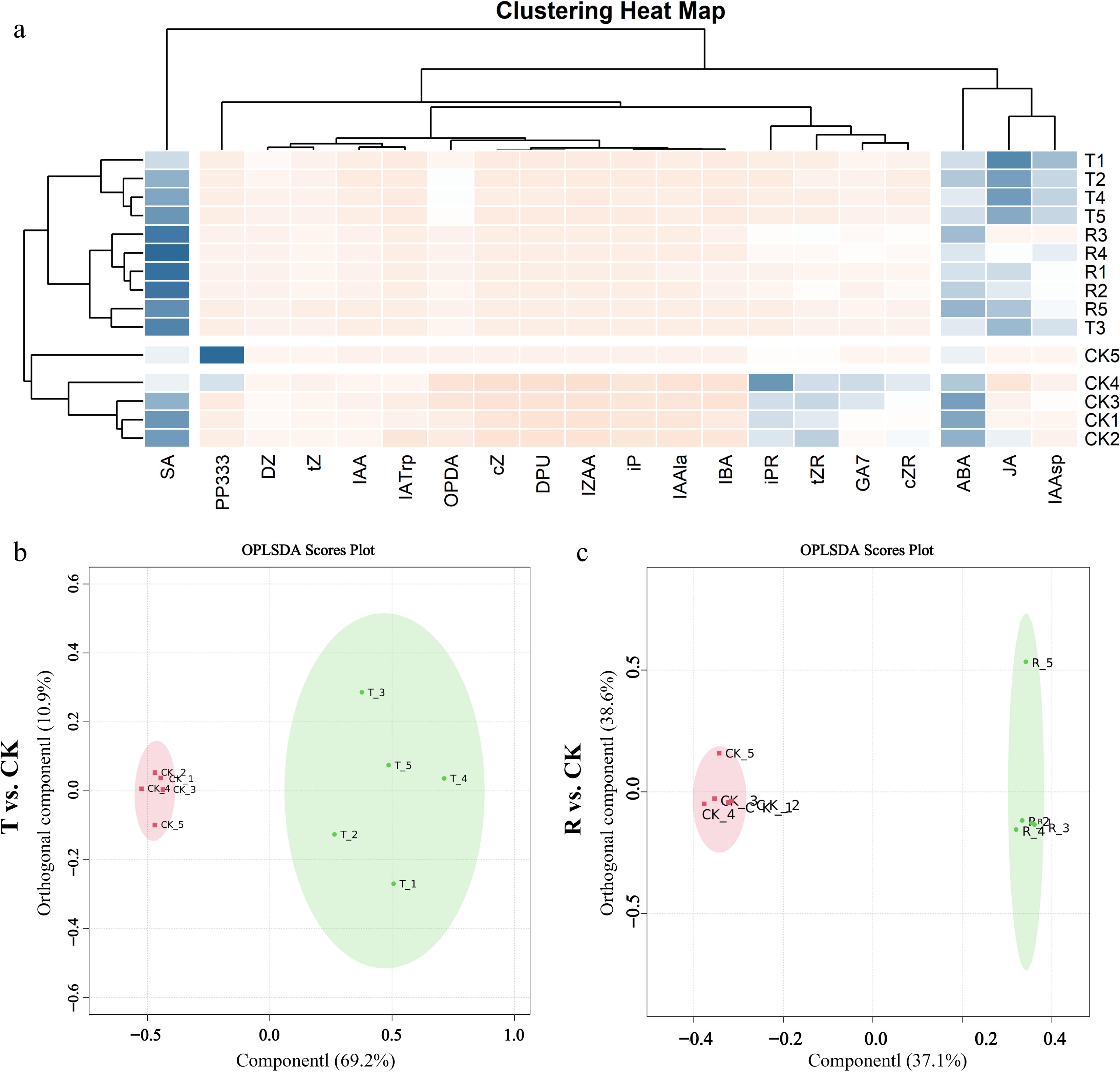
Figure 3.
Heat map of effects of defoliant on plant hormone content in leaves. (a) Differences in hormone content among different treatments. (b) T vs CK OPLS-DA analysis. (c) R vs CK OPLS-DA analysis.
-
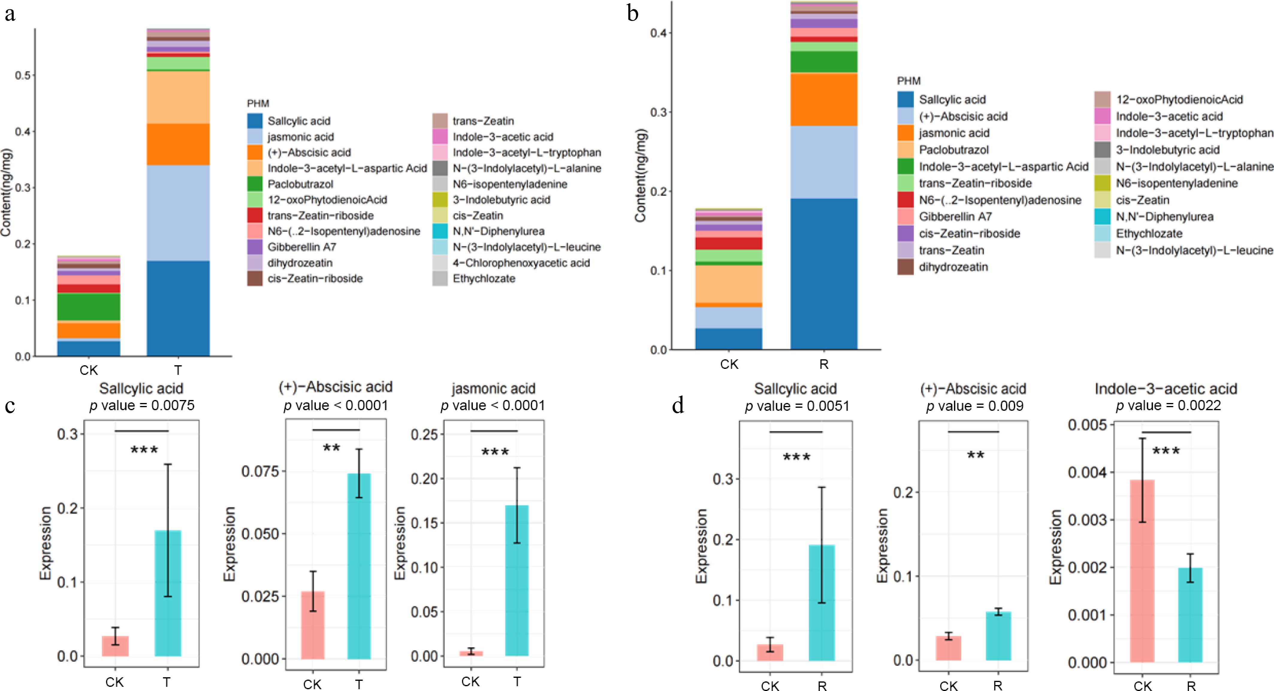
Figure 4.
Effect of defoliant on plant hormone content in leaves. (a) Effect of treatment T on phytohormones in apple leaves. (b) Effect of treatment R on phytohormones in apple leaves. (c) Content of the top three most significantly altered hormones in apple leaves under treatment T. (d) Content of the top three most significantly altered hormones in apple leaves under treatment R. The number of * indicates significant differences between treatments. ** p < 0.05, *** p < 0.001.
-
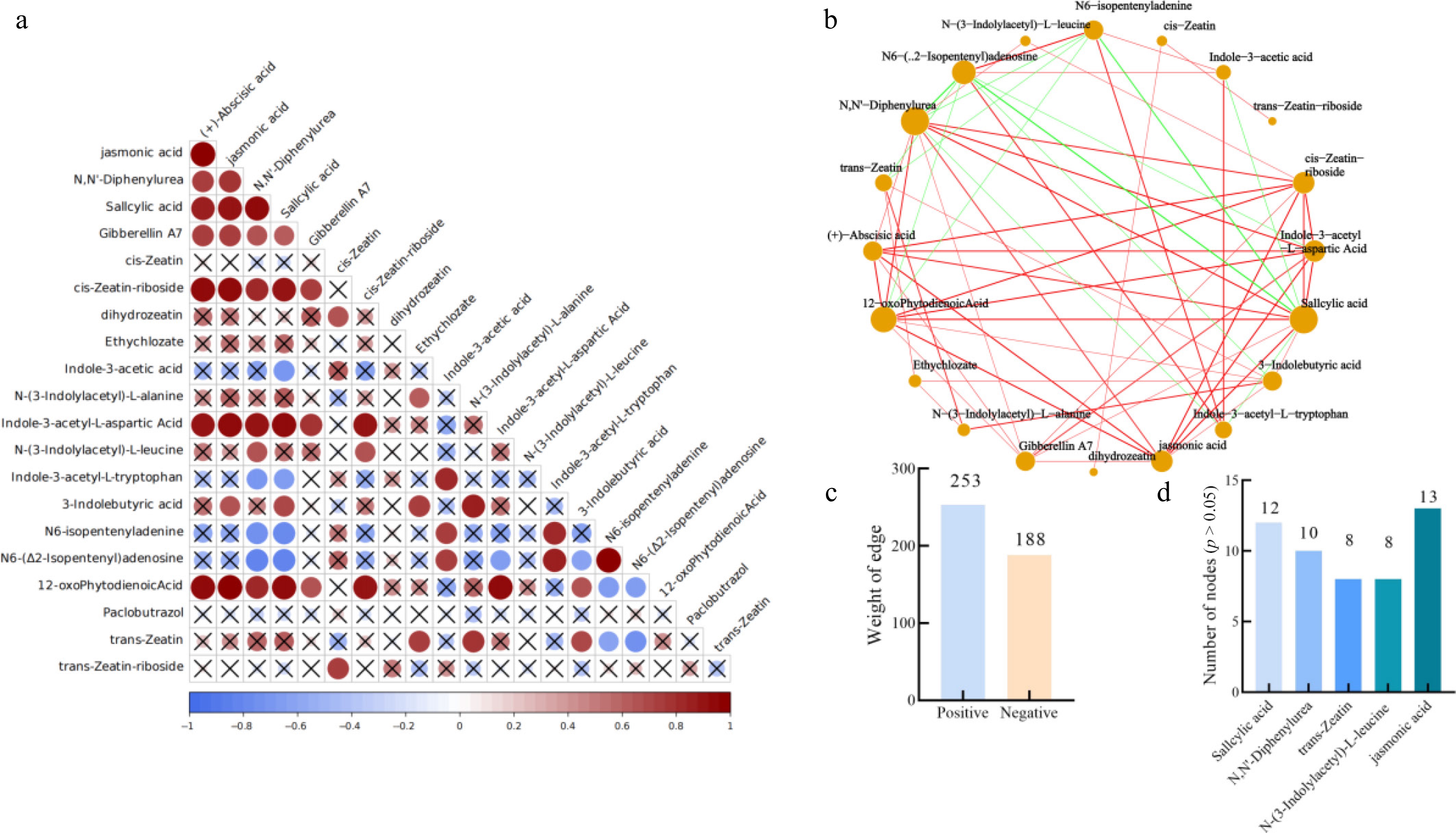
Figure 5.
Correlation between R and CK processing. (a) Correlation among phytohormones in apple leaves under treatment R. (b) Correlation network of phytohormones in apple leaves under treatment R. (c) Edge attributes of the collinearity network. (d) Key nodes with no significant difference (p > 0.05) between treatment R and CK.
-
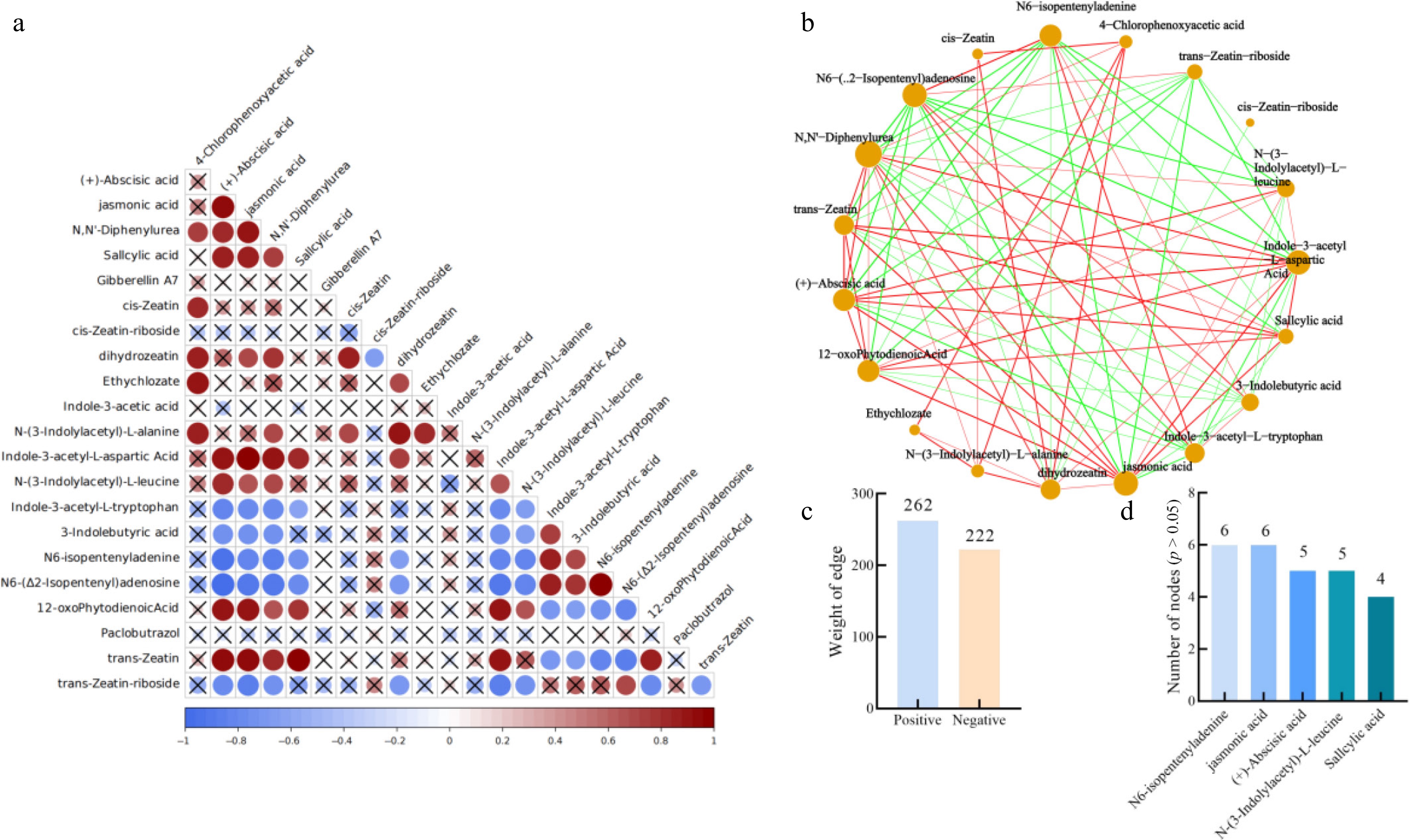
Figure 6.
Correlation between T and CK processing. (a) Correlation among phytohormones in apple leaves under treatment T. (b) Correlation network of phytohormones in apple leaves under treatment T. (c) Edge attributes of the collinearity network. (d) Key nodes with no significant difference (p > 0.05) between Treatment T and CK.
-
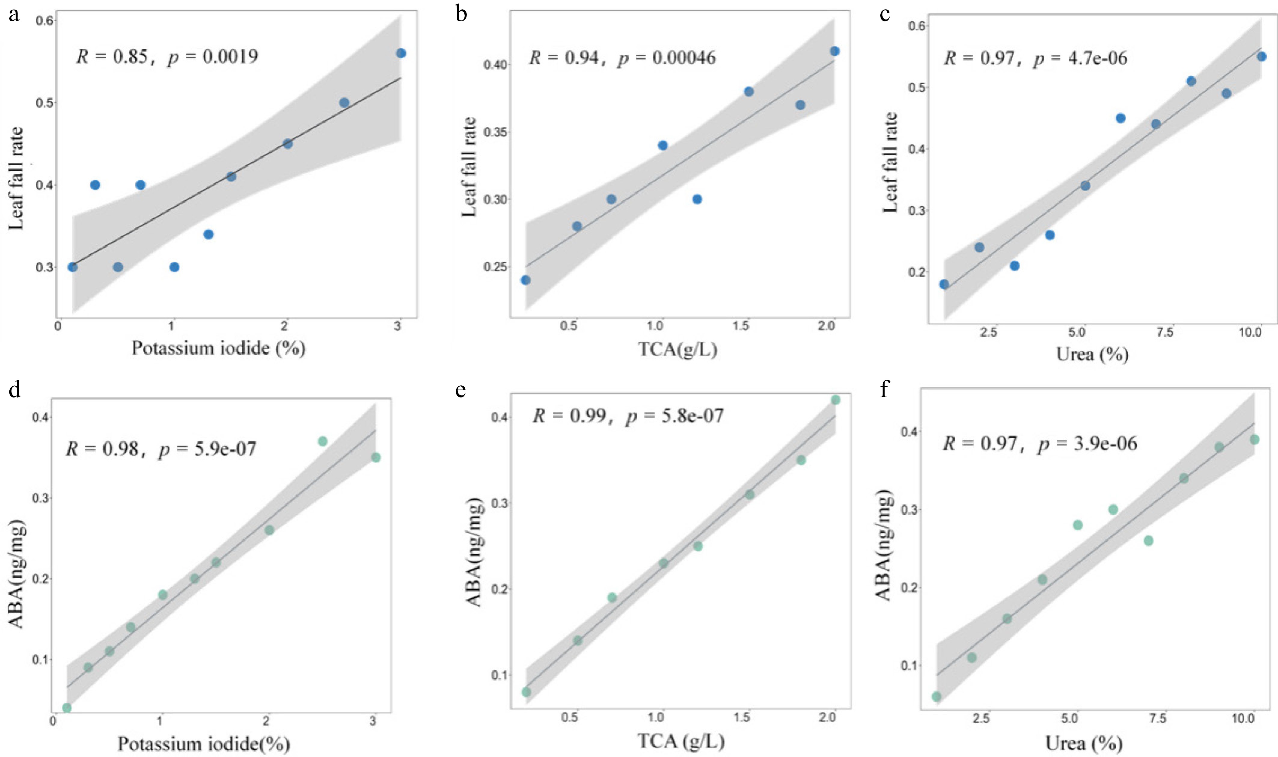
Figure 7.
Correlation analysis of defoliant content with leaf fall rate and ABA content.
-
No. A: Urea (%) B: KI (%) C: TCA (g·L−1) Leaf fall rate 1 5.00 0.40 1.50 0.57 2 2.00 0.40 1.00 0.32 3 5.00 0.30 1.00 0.49 4 2.00 0.20 1.00 0.12 5 8.00 0.40 1.00 0.19 6 5.00 0.30 1.00 0.50 7 5.00 0.30 1.00 0.60 8 8.00 0.20 1.00 0.35 9 5.00 0.30 1.00 0.52 10 5.00 0.20 0.50 0.50 11 5.00 0.20 1.50 0.48 12 5.00 0.30 1.00 0.57 13 2.00 0.30 0.50 0.30 14 8.00 0.30 0.50 0.39 15 5.00 0.40 0.50 0.49 16 2.00 0.30 1.50 0.34 17 8.00 0.30 1.50 0.32 Table 1.
Experimental design and results of response surface.
-
Source of variation Quadratic sum Degree of freedom Mean sum of square F P Model 0.2927 9.0000 0.0325 25.1200 0.0002 Significant A 0.0042 1.0000 0.0042 3.2100 0.1162 B 0.0020 1.0000 0.0020 1.5700 0.2505 C 0.0001 1.0000 0.0001 0.0542 0.8225 AB 0.0309 1.0000 0.0309 23.8300 0.0018 AC 0.0026 1.0000 0.0026 2.0000 0.1997 BC 0.0027 1.0000 0.0027 2.0500 0.1995 Residual 0.0091 7.0000 0.0013 Lack of fit 0.0009 3.0000 0.0003 0.1551 0.9211 Not significant Pure error 0.0081 4.0000 0.0020 Cor error 0.3017 16.0000 Table 2.
Analysis of model variance.
-
Standard deviation
(R2)Average
(R2 correction)Coefficient
(R2 prediction)Signal-to-
noise ratio0.97 0.93 0.91 15.87 Table 3.
R2 comprehensive analysis.
Figures
(7)
Tables
(3)