-
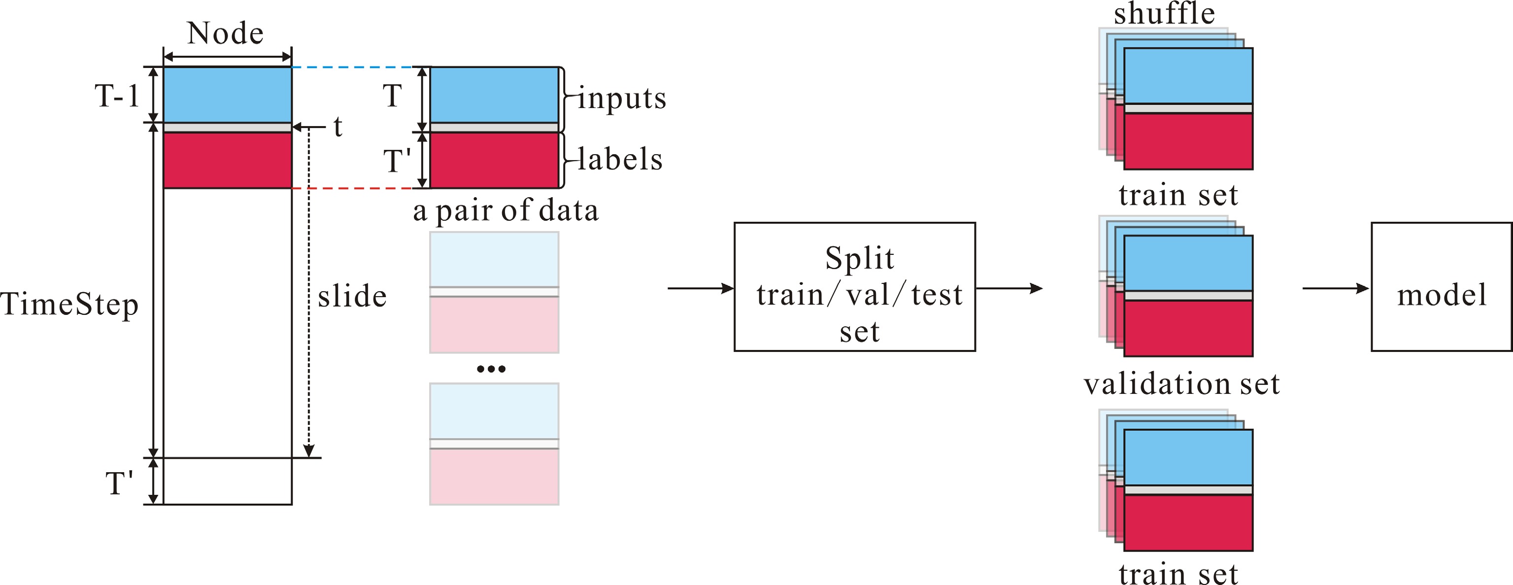
Figure 1.
Data preprocessing steps.
-
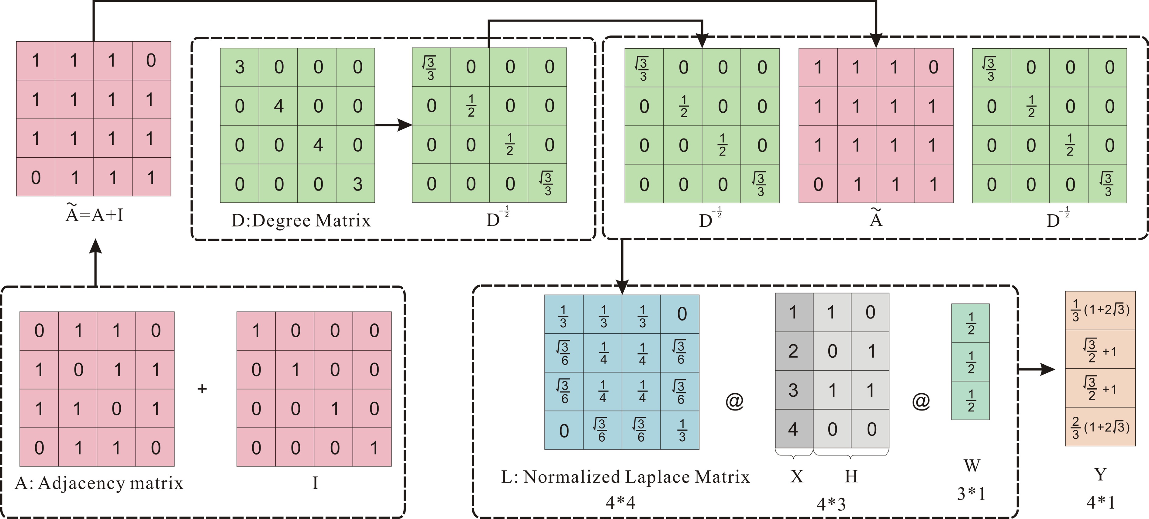
Figure 2.
Graph convolution.
-
Figure 3.
DCRNN: diffusion convolution for spatial dependencies, GRU for temporal dependencies.
-
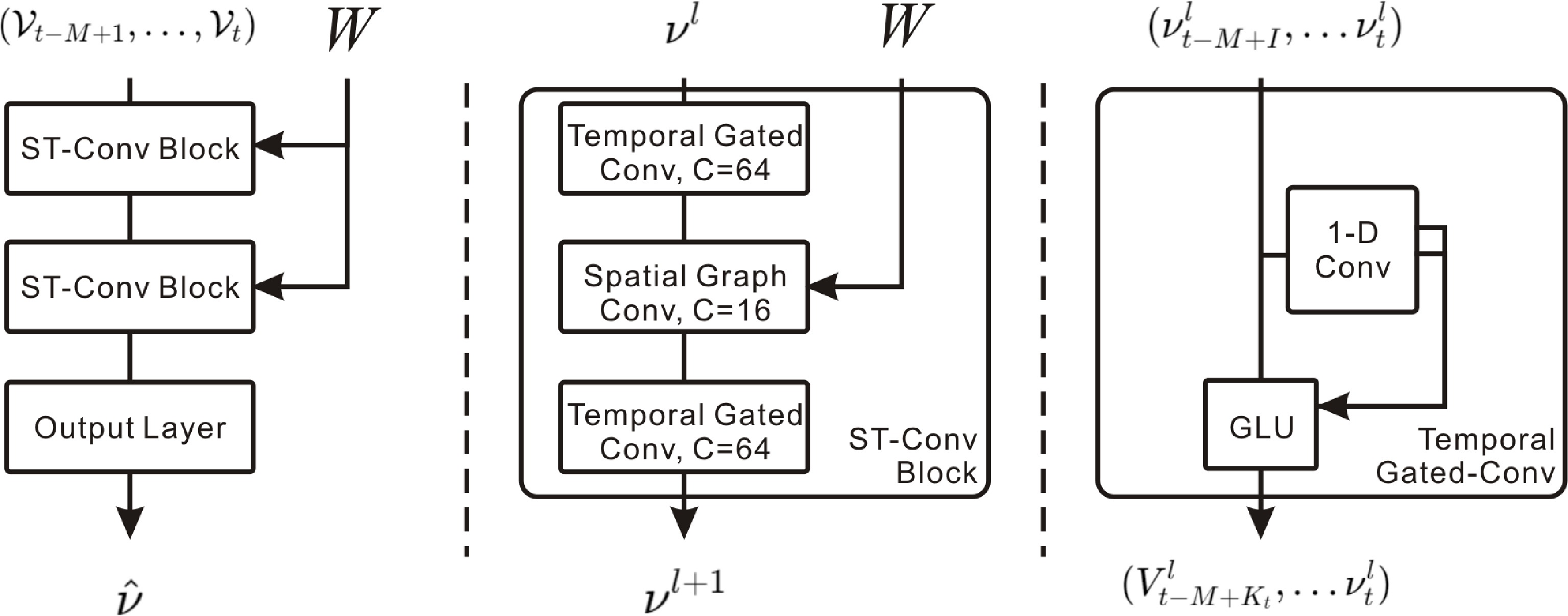
Figure 4.
STGCN: combines spectral graph convolution for spatial features and gated causal CNN for temporal features.
-
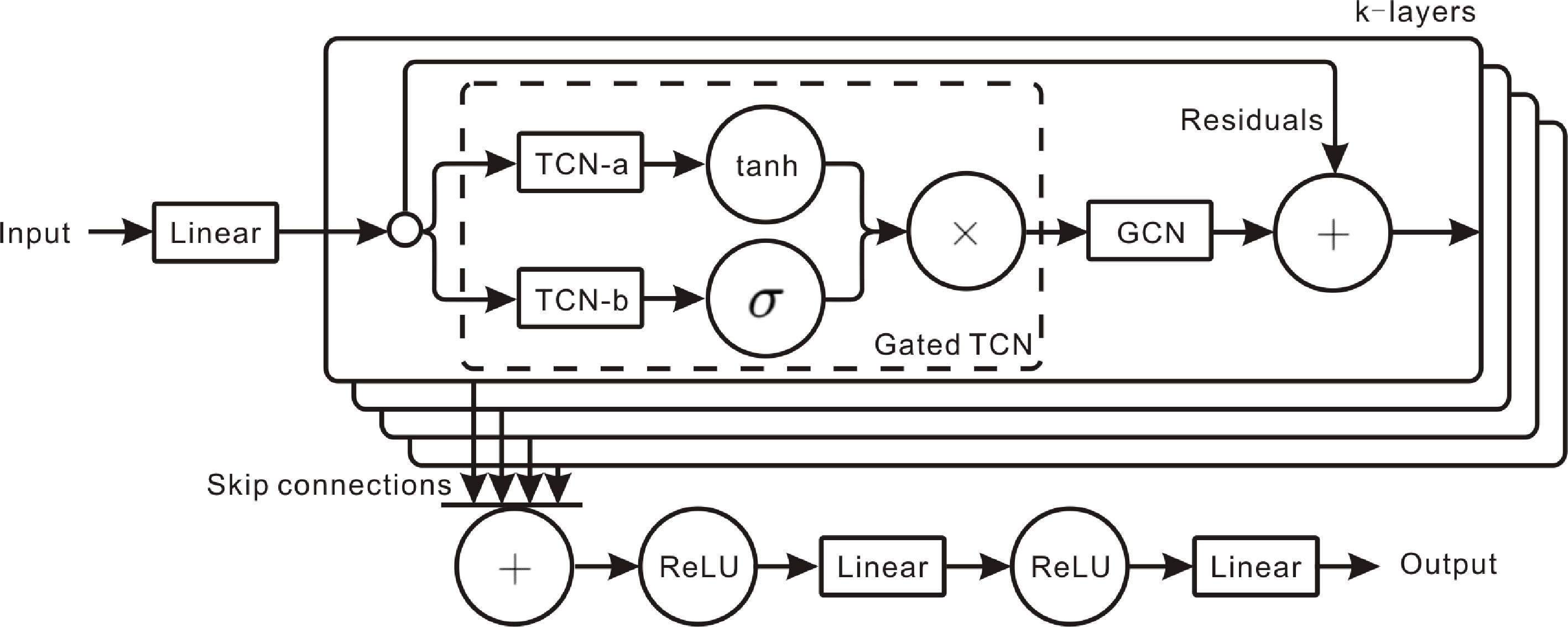
Figure 5.
Graph WaveNet: adaptive adjacency captures spatial relations, while dilated causal convolution models temporal dynamics.
-

Figure 6.
STSGCM: captures local spatiotemporal correlations via a spatial-temporal synchronous graph convolution module.
-
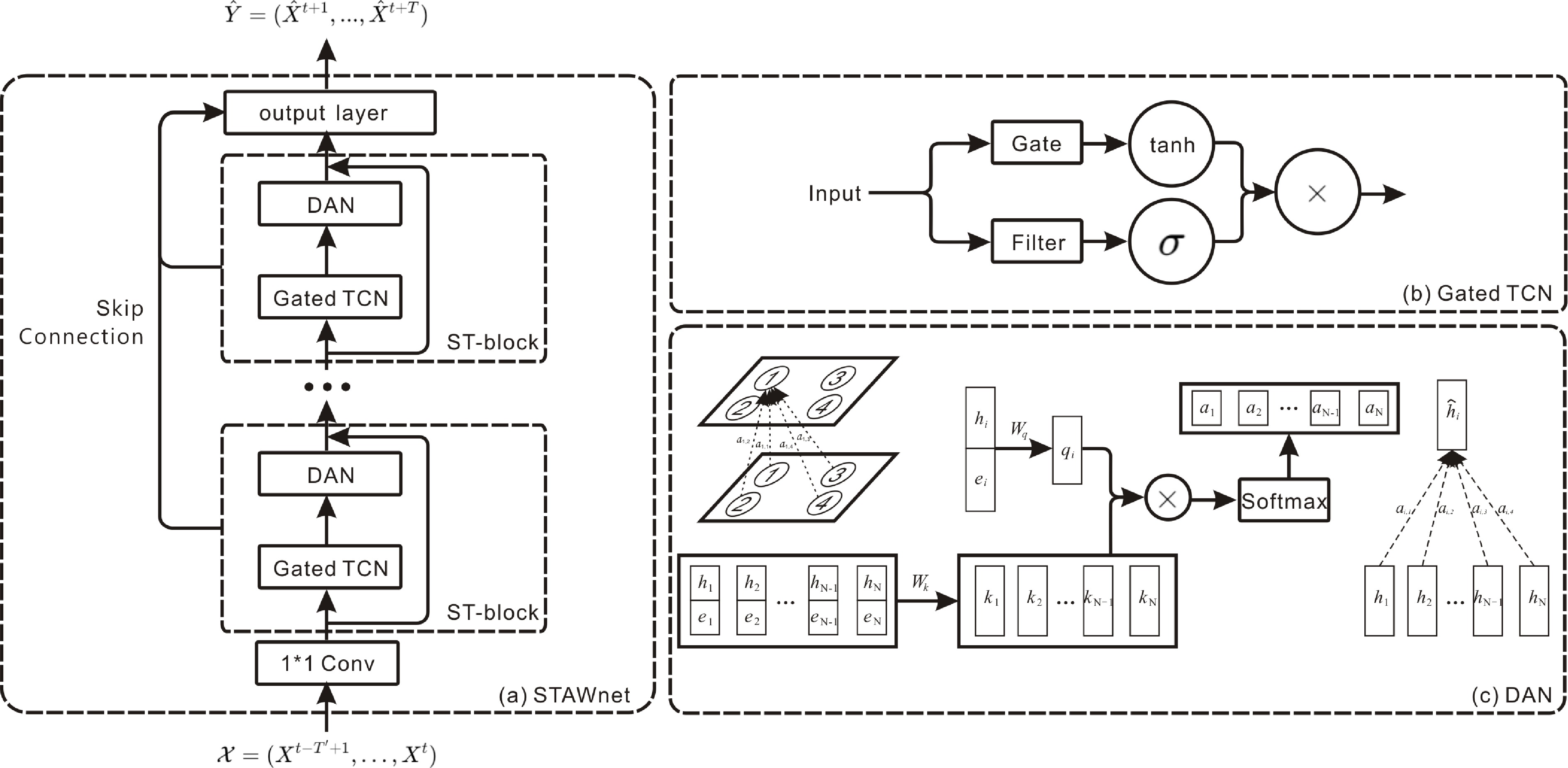
Figure 7.
STAWnet: self-learned node embeddings capture hidden spatial dependencies, while temporal convolution and dynamic attention capture temporal dynamics.
-
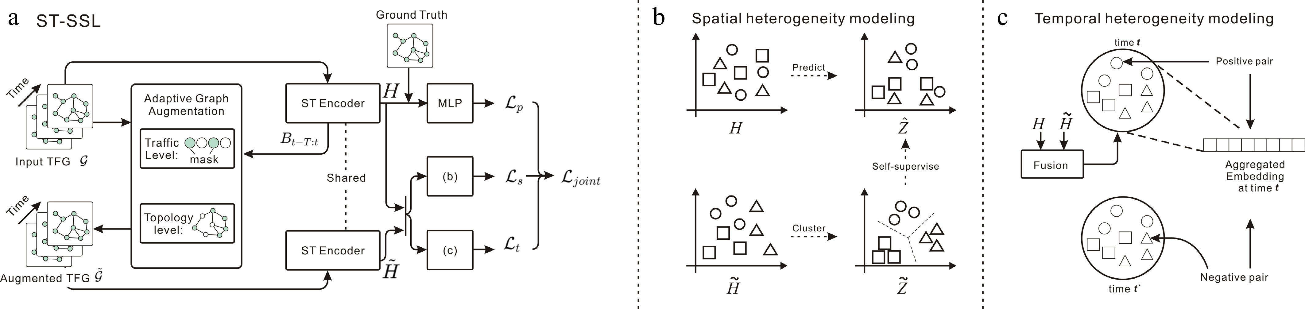
Figure 8.
ST-SSL: integrates temporal and spatial convolutions for spatiotemporal patterns, enhanced by self-supervised tasks for spatial-temporal heterogeneity.
-
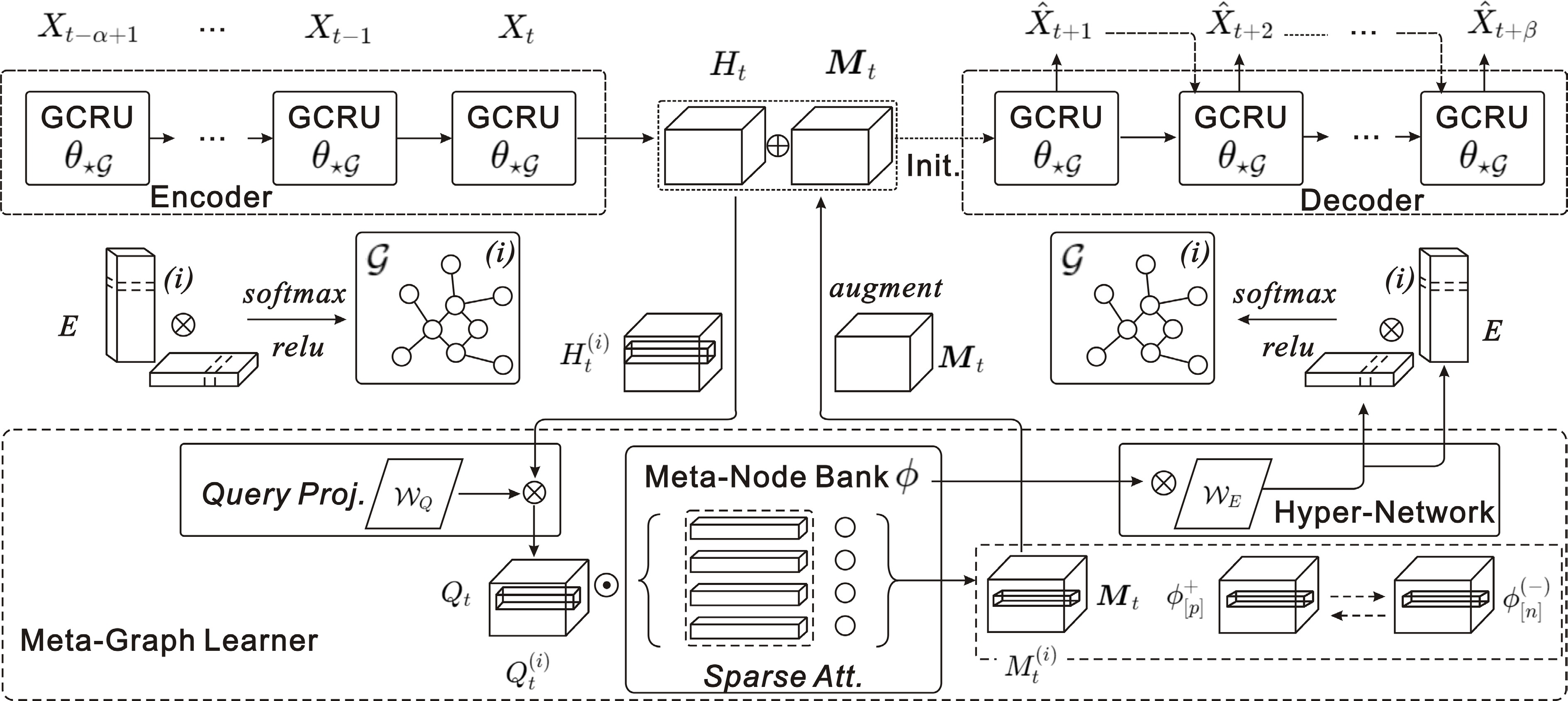
Figure 9.
MegaCRN: meta-graph learner dynamically generates node embeddings capturing spatiotemporal nuances, integrated with a GCRN for prediction.
-
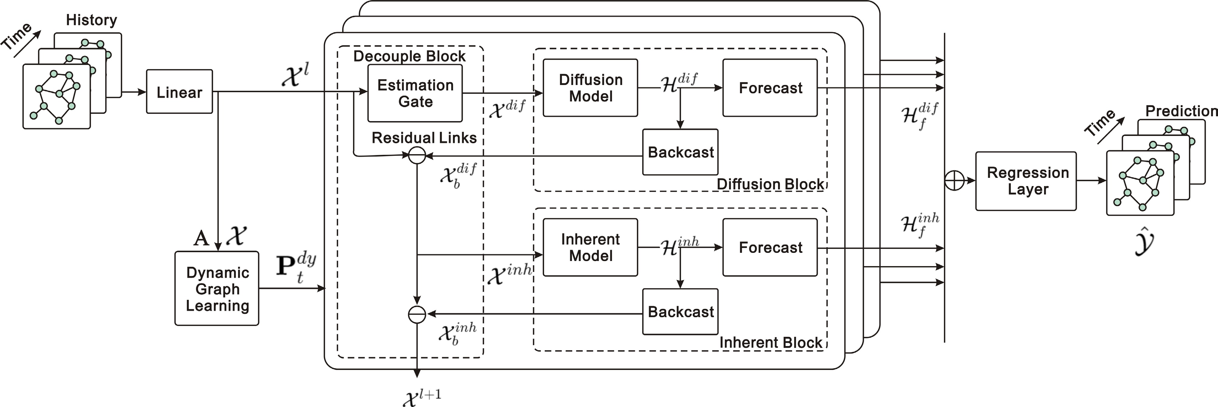
Figure 10.
D2STGNN: decouples diffuse and intrinsic signals via a decoupled spatiotemporal framework with dynamic graph learning.
-
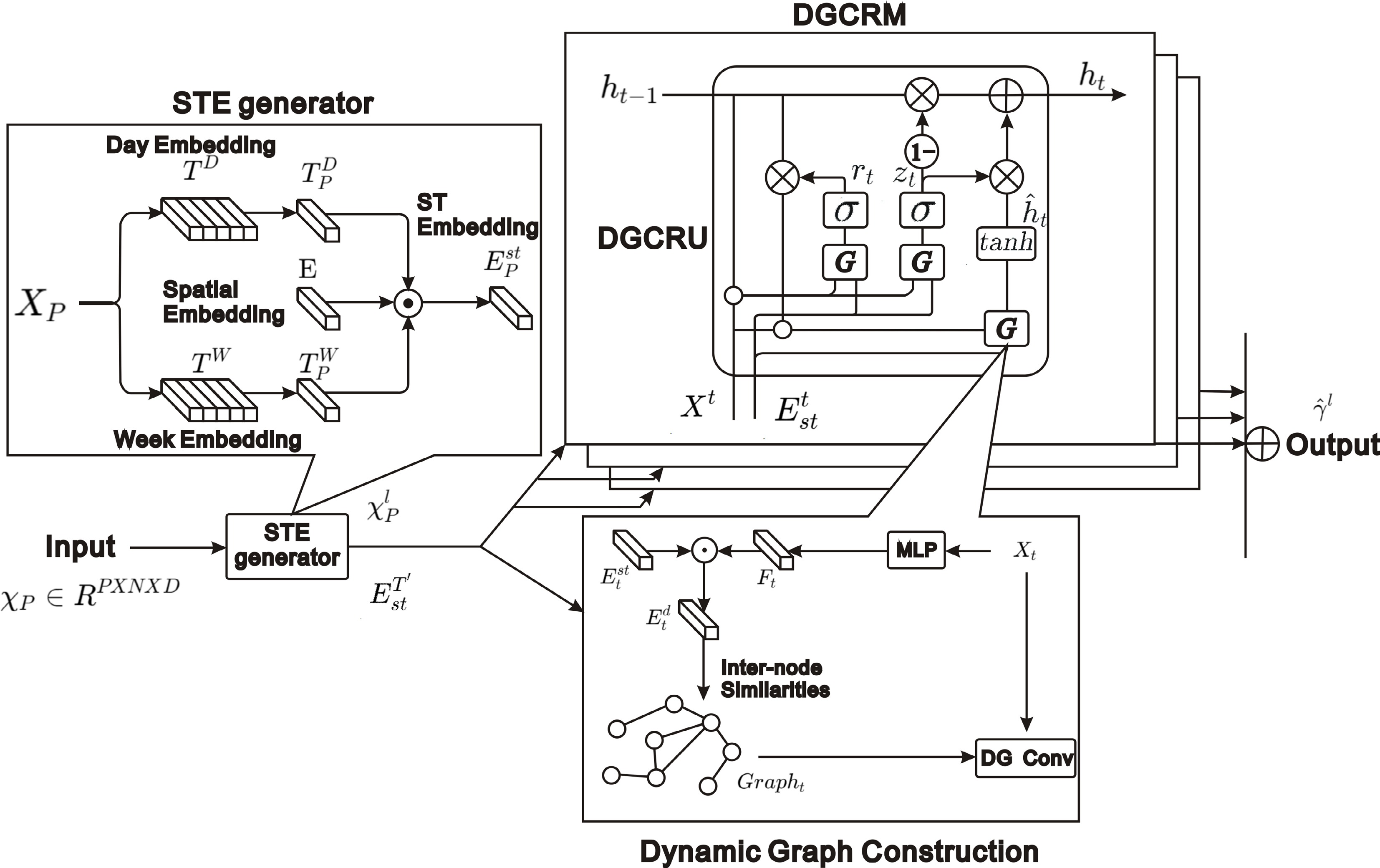
Figure 11.
DDGCRN: dynamically generates graphs from traffic signals and uses DGCRM to capture spatiotemporal features efficiently.
-
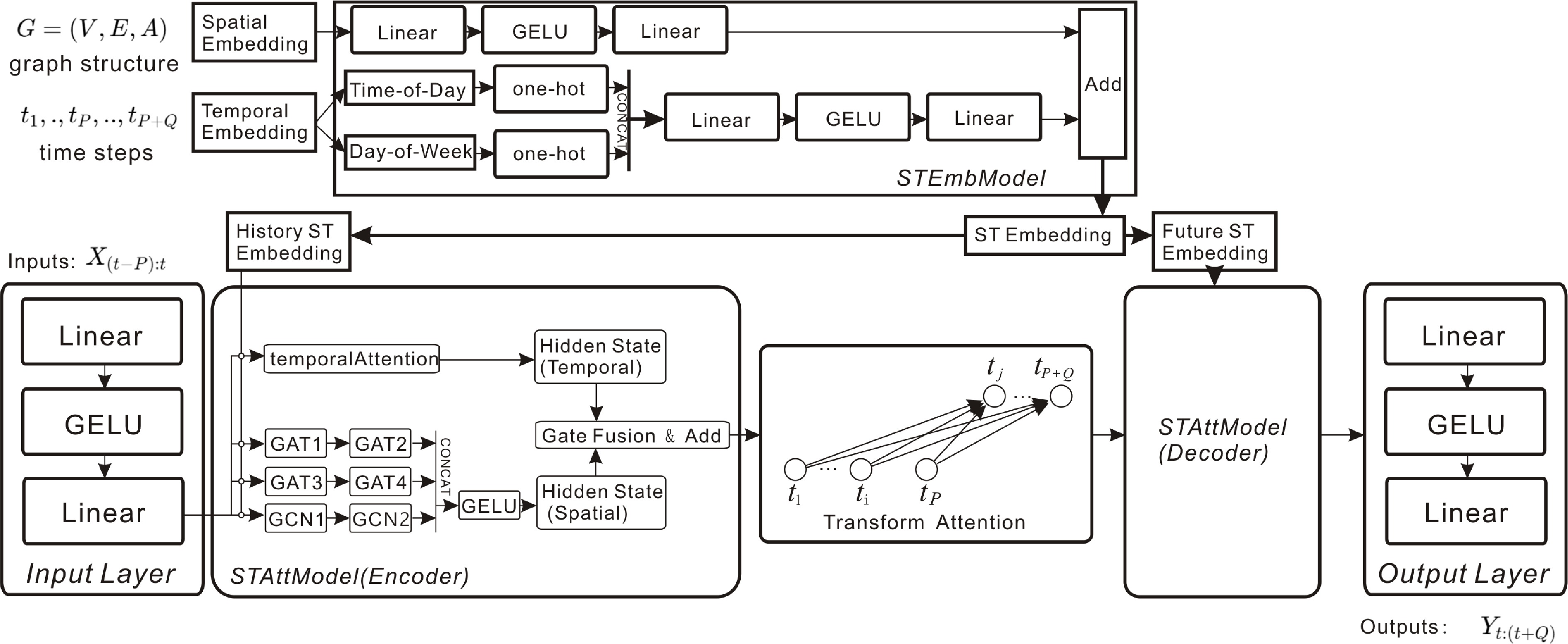
Figure 12.
RGDAN: random GAT with adaptive matrix captures spatial dependencies, while temporal attention captures time-related patterns.
-
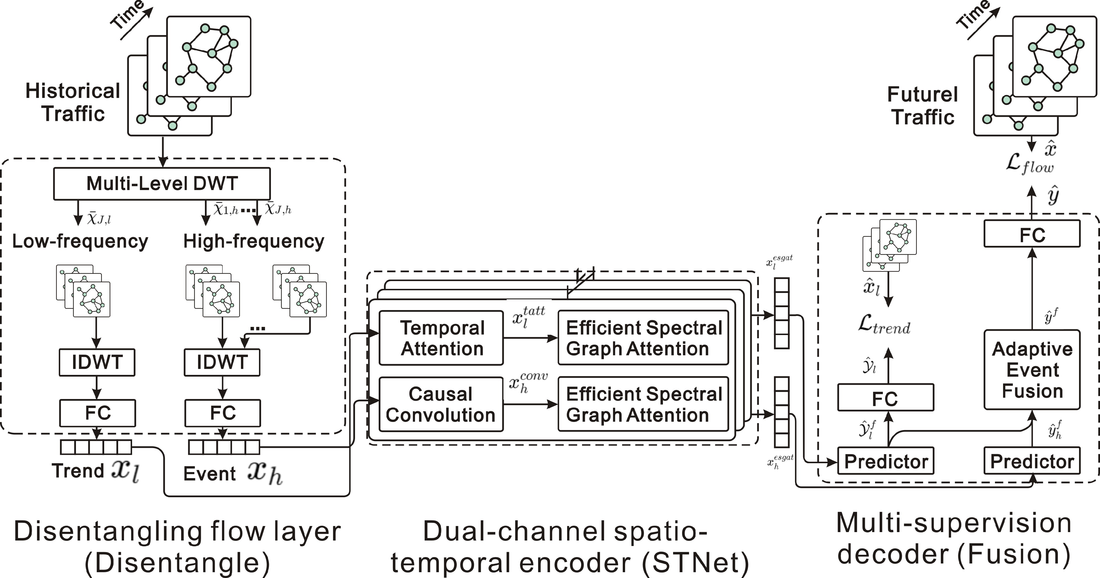
Figure 13.
STWave: decouples traffic series into trends and events with DWT, and uses dual-channel spatiotemporal network and ESGAT for modeling.
-
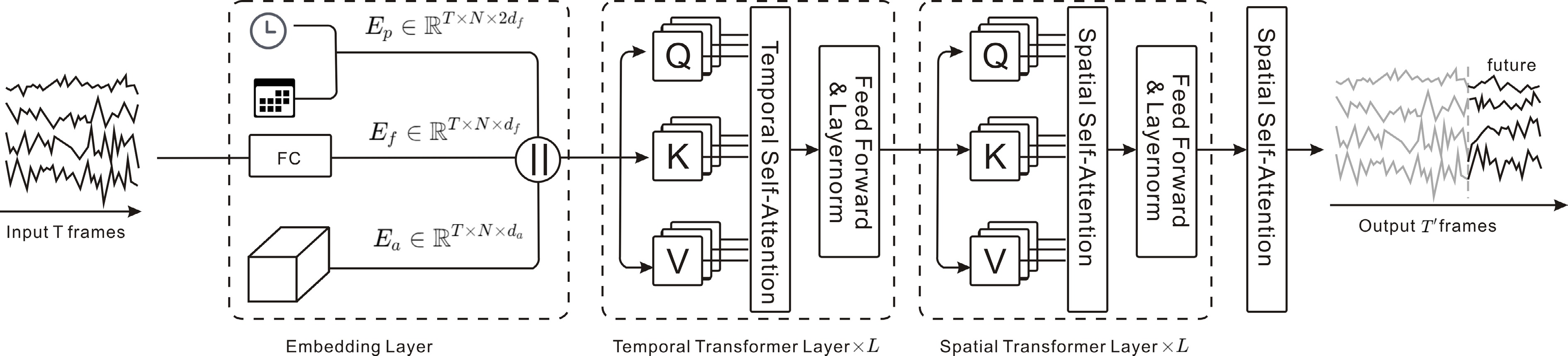
Figure 14.
STAEFormer: spatiotemporal adaptive embedding enhances Transformer to capture complex spatiotemporal dynamics in traffic data.
-
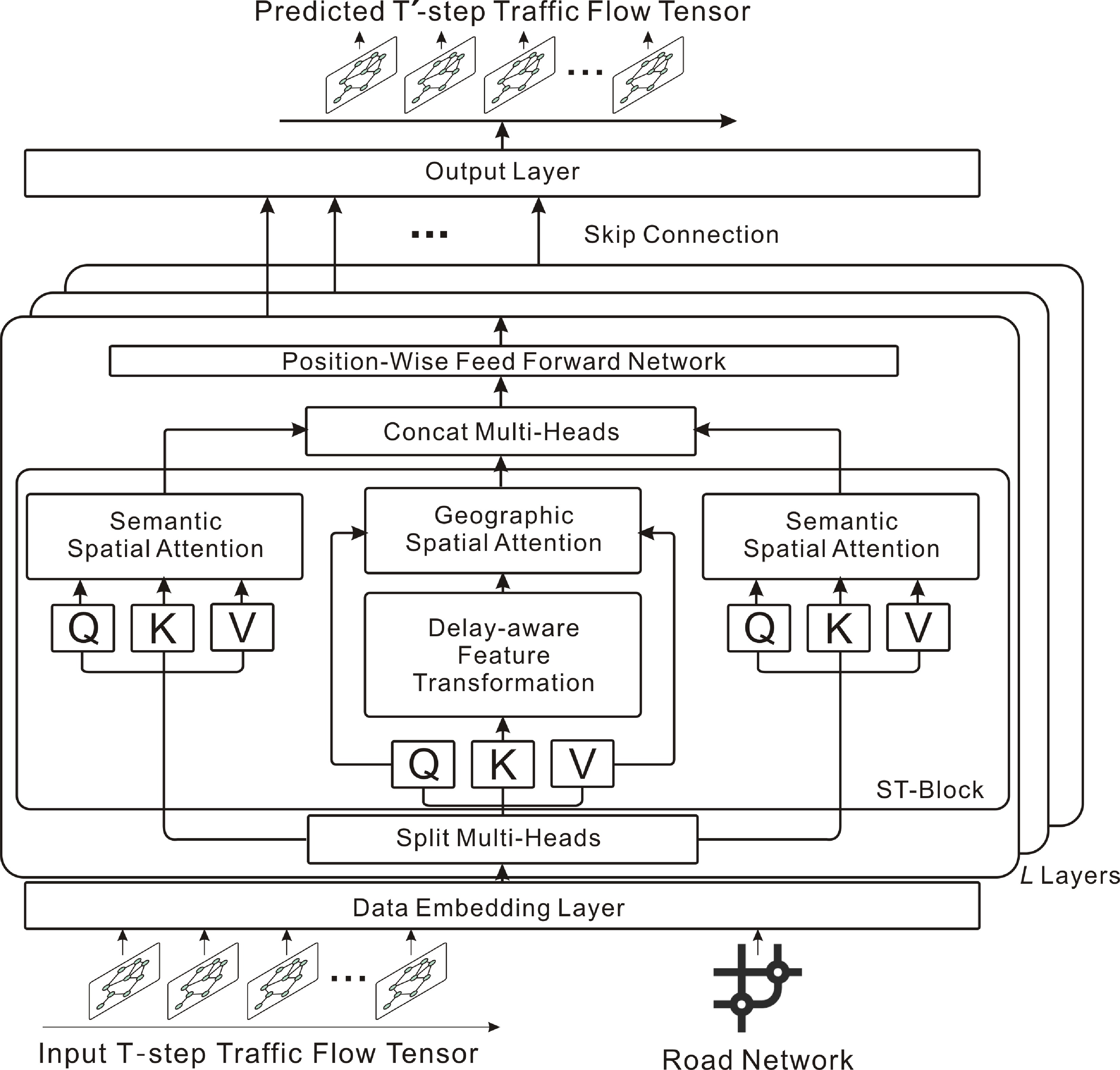
Figure 15.
PDFormer: spatial self-attention, graph masking, and delay-aware transformation model complex spatiotemporal dependencies.
-

Figure 16.
STEP: Pre-training on long-term traffic sequences provides segment-level representations to enhance STGNN predictions.
-
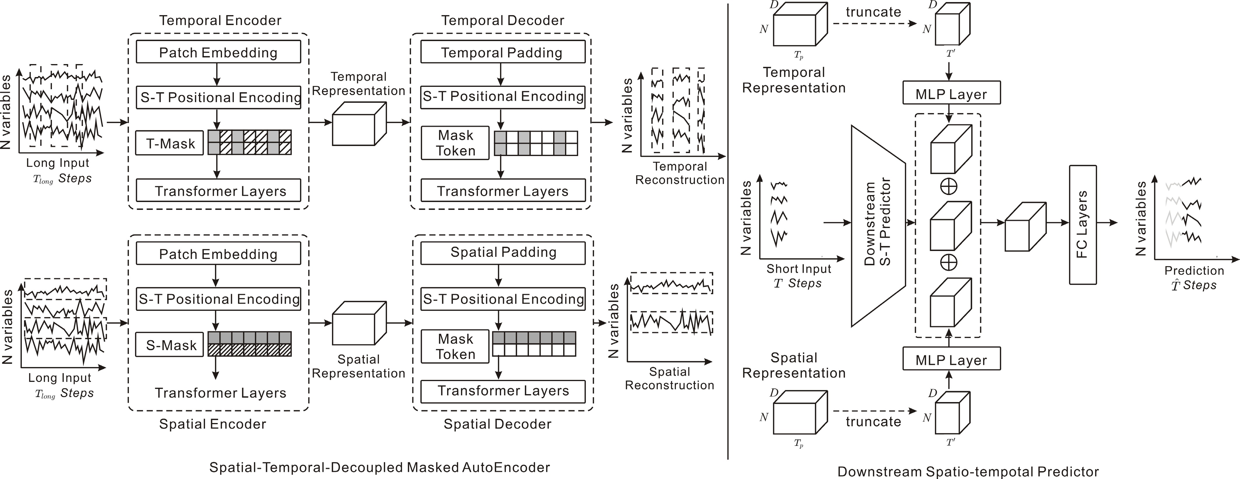
Figure 17.
STD-MAE: Decoupled spatial-temporal masked autoencoders reconstruct sequences to capture long-range heterogeneity in traffic data.
-
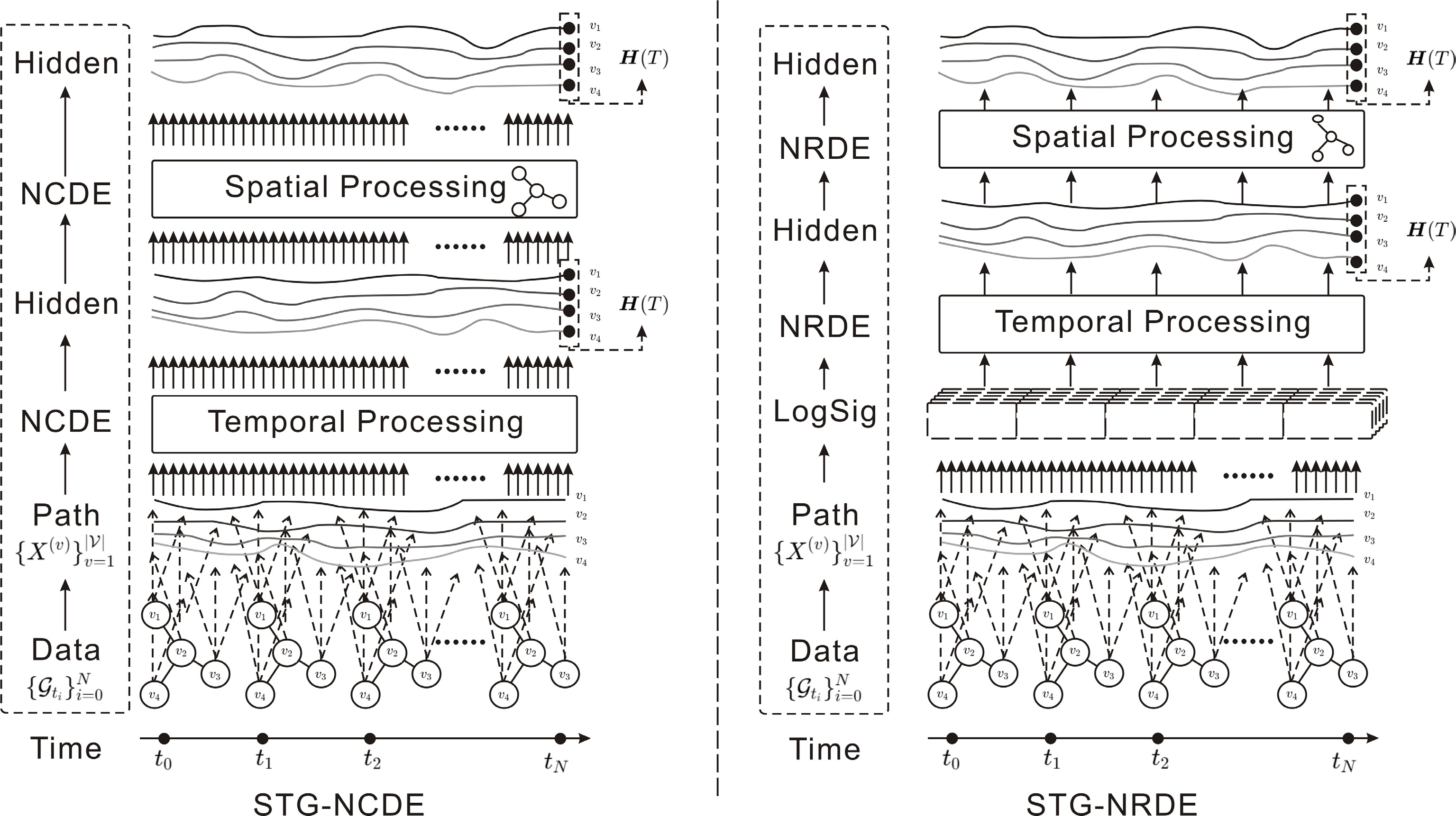
Figure 18.
STG-NCDE and STG-NRDE: Temporal and spatial NCDEs/NRDEs jointly model continuous-time dynamics and intricate patterns in traffic flows.
-
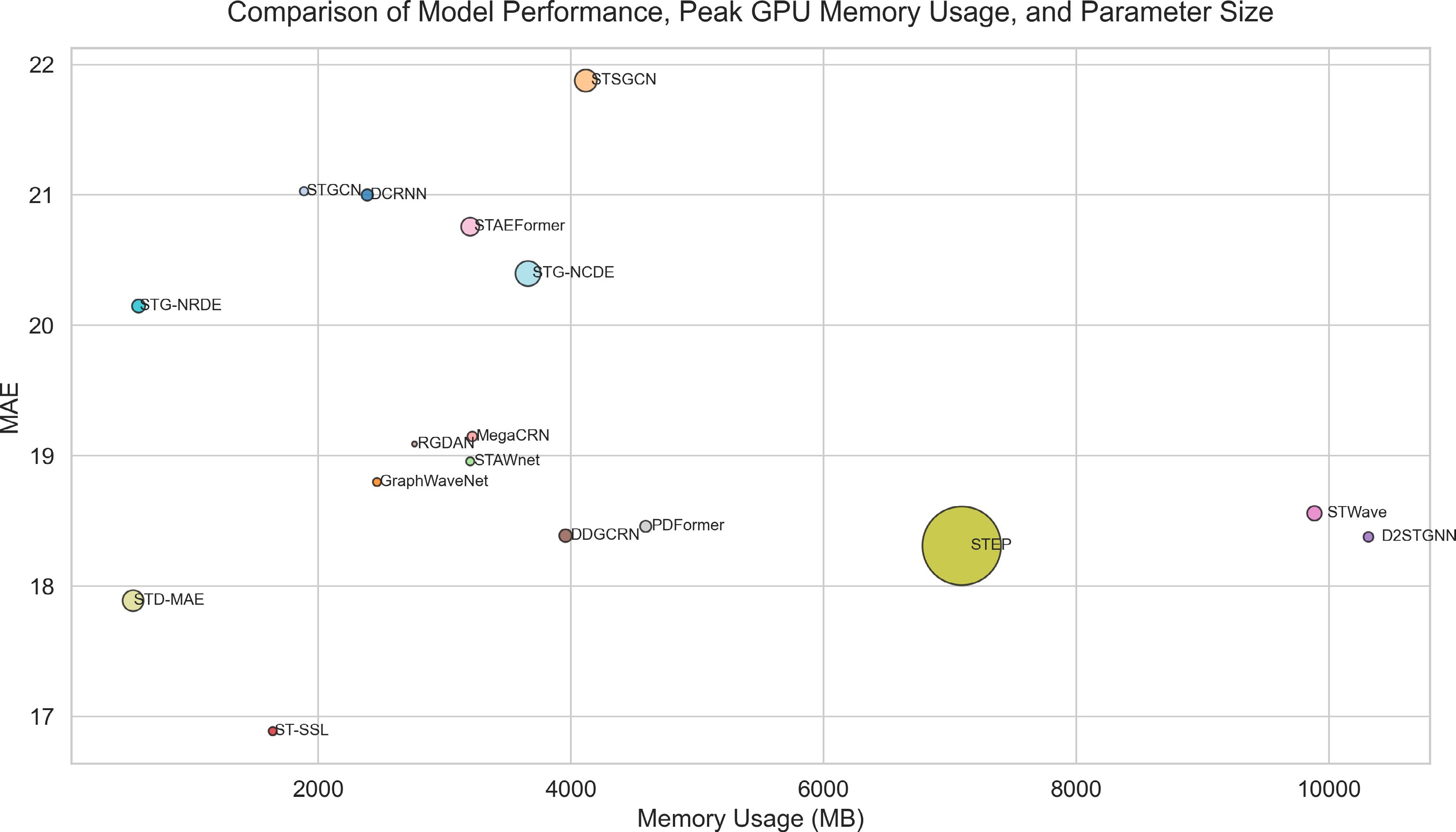
Figure 19.
Model performance vs memory and parameters.
-
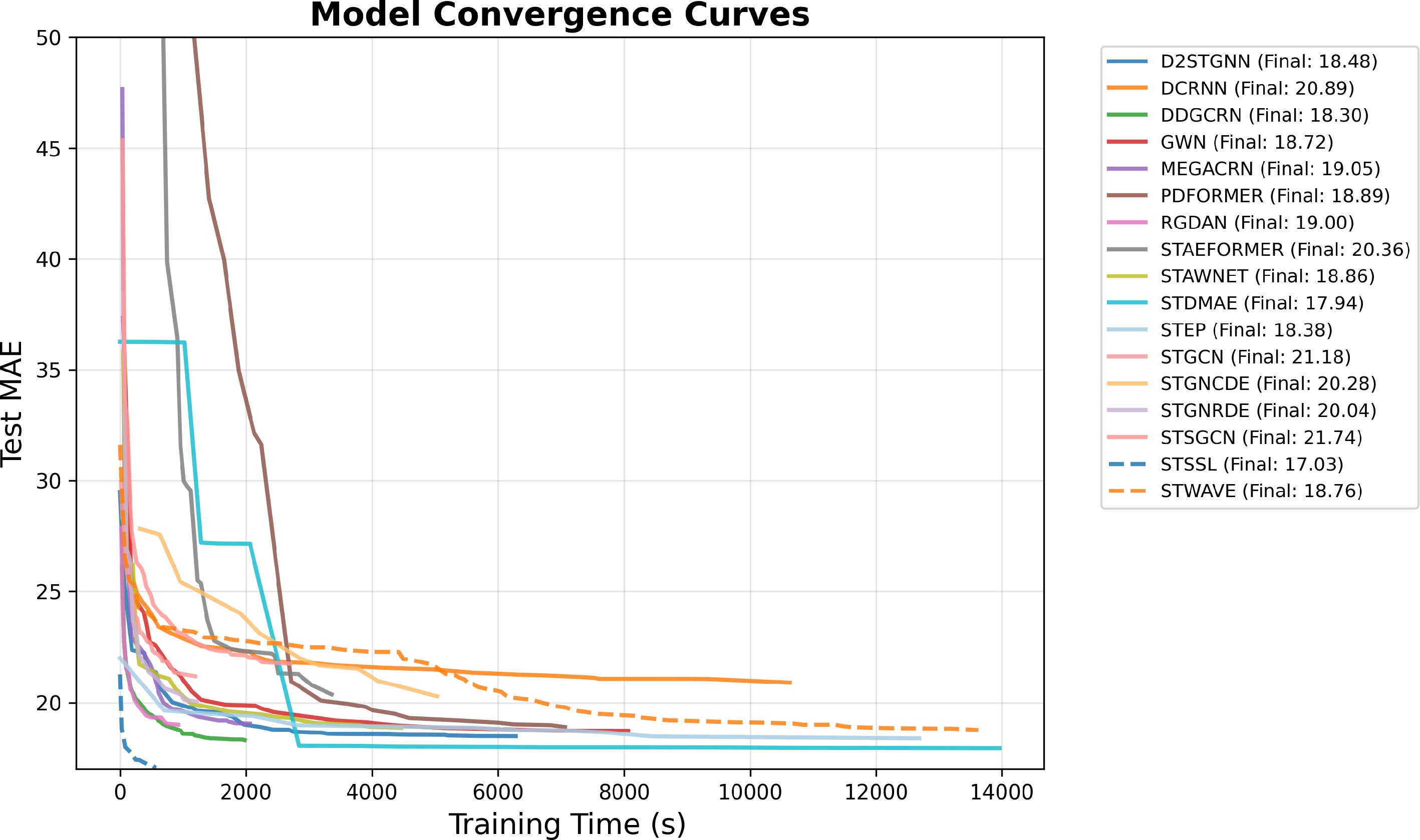
Figure 20.
Training convergence curves of MAE over time.
-
Model Tag Source Year DCRNN[49] RNN/GNN ICLR 2018 2018 STGCN[50] CNN/GCN IJCAI 2018 2018 GraphWaveNet[51] TCN/GCN IJCAI 2019 2019 STSGCN[52] GCN AAAI 2020 2020 STAWnet[53] TCN IET intelligent transport systems 2021 ST-SSL[54] GCN AAAI 2023 2023 MegaCRN[55] RNN/GCN AAAI 2023 2023 D2STGNN[56] CNN/GCN VLDB 2022 2022 DDGCRN[57] GCN Pattern recognition 2023 RGDAN[58] GAT Neural networks 2024 STWave[59] GAT ICDE 2023 2023 STAEformer[60] Transformer CIKM 2023 2023 PDFormer[61] Transformer AAAI 2023 2023 STEP[62] Pre-training SIGKDD 2022 2022 STDMAE[63] Pre-training IJCAI 2024 2024 STG-NCDE[64] Differential equations AAAI 2022 2022 STG-NRDE[65] Differential equations ACM transactions on intelligent systems and technology 2023 Table 1.
Model list.
-
Dataset Nodes Edges Time range Sample rate Zero value rate Type METR-LA 207 1,515 2012/03/01−2012/06/30 5 min 7.581% Speed PEMS-BAY 325 2,369 2017/01/01−2017/05/31 5 min 4.906% Speed PeMSD7(M) 228 1,664 2012/05/01−2012/06/30 5 min 0.10% Speed PeMSD7(L) 1,026 14,534 2012/05/01−2016/06/30 5 min 0.50% Speed PEMS03 358 546 2018/09/01−2018/11/30 5 min 5.102% Flow PEMS04 307 338 2018/01/01−2018/02/28 5 min 5.730% Flow PEMS07 883 865 2017/01/05−2017/08/06 5 min 5.028% Flow PEMS08 170 276 2016/07/01−2016/08/31 5 min 5.070% Flow CA 8,600 201,363 2017/01/01−2021/12/31 15 min 5.869% Flow GLA 3,834 98,703 2017/01/01−2021/12/31 15 min 5.712% Flow GBA 2,352 61,246 2017/01/01−2021/12/31 15 min 5.719% Flow SD 716 17,319 2017/01/01−2021/12/31 15 min 5.845% Flow NYC-taxi 16*12 − 2016/01/01−2016/02/29 30 min 48.63% Inflow/outflow NYC-bike 14*8 − 2016/08/01−2016/09/29 30 min 52.55% Inflow/outflow SZ-taxi 156 532 2015/01/01−2015/01/31 15 min 26.57% Speed Table 2.
Datasets overview.
-
Device Info CPU Intel(R) Xeon(R) Gold 6133 CPU @ 2.50GHz GPU NVIDIA GeForce RTX 4090 RAM 32 GB VRAM 24 GB Python 3.10.16 CUDA 12.3 PyTorch 2.6.0 Table 3.
Device information.
-
Model Params MAE RMSE MAPE VRAM RAM Iter per second HA − 38.03 59.24 27.88 − − − ARIMA − 33.73 48.80 24.18 − − − VAR − 24.54 38.61 17.24 − − − DCRNN 546,881 21.00 33.16 14.66 2,385.22 1,276.96 3.09 STGCN 297,228 21.03 33.38 15.07 1,886.88 1,177.90 14.30 GraphWaveNet 278,632 18.80 30.87 12.38 2,461.48 1,241.01 5.46 STSGCN 2,024,445 21.88 35.49 15.29 4,114.91 1,028.78 7.09 STAWnet 281,756 18.96 31.35 12.72 3,200.94 1,254.59 5.21 ST-SSL 288,275 16.89 26.98 10.48 3,208.00 1,566.00 16.19 MegaCRN 392,761 19.15 31.36 12.58 3,217.96 1,140.38 7.72 D2STGNN 398,788 18.38 30.10 12.06 10,310.0 5,067.00 6.34 DDGCRN 671,704 18.39 30.73 12.09 3,957.25 1,441.35 8.38 RGDAN 107,285 19.09 32.10 12.99 2,759.20 1,164.68 19.12 STWave 882,558 18.56 30.36 12.81 9,884.15 4,712.99 2.17 STAEFormer 1,354,932 20.76 32.38 20.06 3,200.36 1,217.37 19.88 PDFormer 531,165 18.46 29.97 12.67 4,591.52 5,351.85 1.64 STEP 25,469,726 18.31 29.90 12.49 7,091.23 1,936.99 2.02 STD-MAE 673,384 17.89 29.33 12.11 532.70 3,628.76 99.72 STG-NRDE 716,628 20.15 32.22 13.51 577.83 3,739.68 5.26 STG-NCDE 2,600,532 20.40 32.30 13.95 3,657.37 3,793.33 0.85 Table 4.
Runtime, resource usage, and predictive performance of models on PEMS04.
-
Training data proportion MAE RMSE MAPE 10% 19.66 31.77 13.08% 30% 20.12 32.54 13.15% 50% 19.87 31.97 13.64% 70% 19.50 31.54 12.66% 100% 18.82 30.78 12.41% Table 5.
Model performance under different training data proportions.
Figures
(20)
Tables
(5)