-
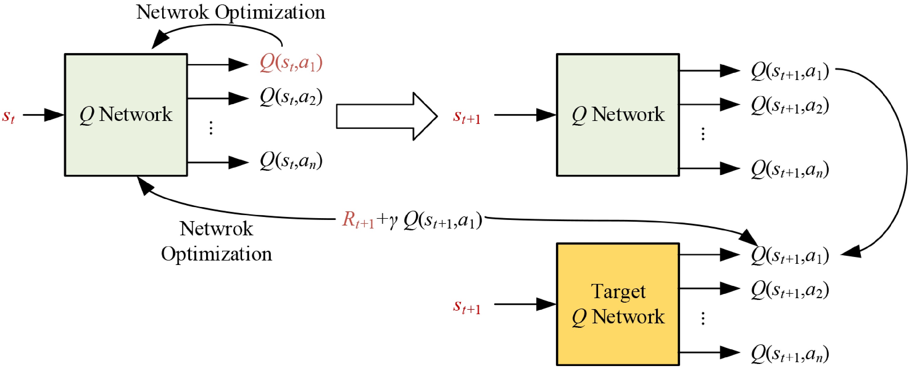
Figure 1.
The update process of DDQN.
-
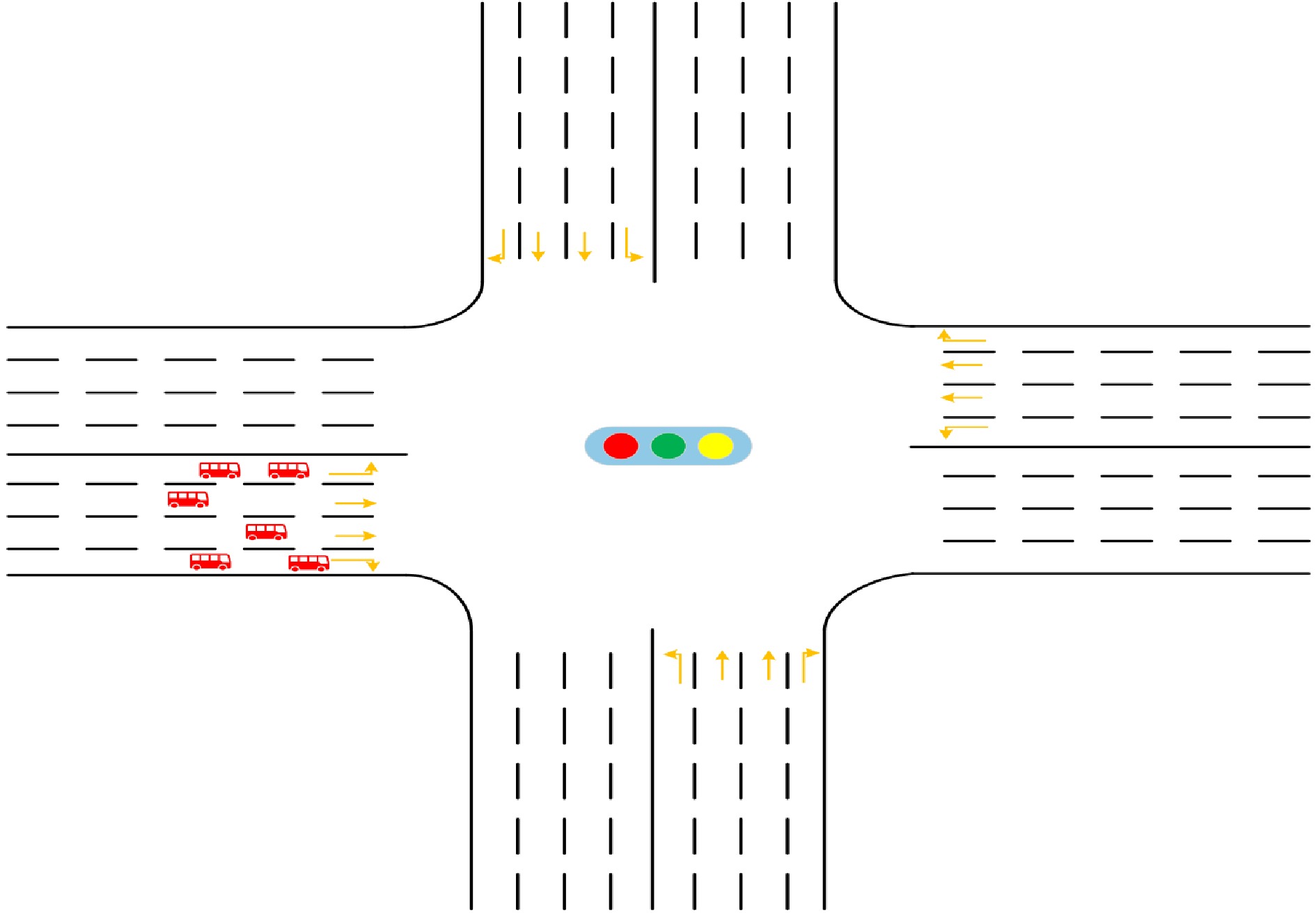
Figure 2.
Typical four-arm signalized intersection.
-
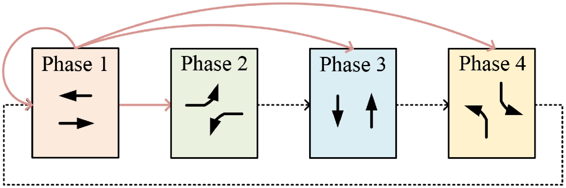
Figure 3.
Signal phase setting.
-
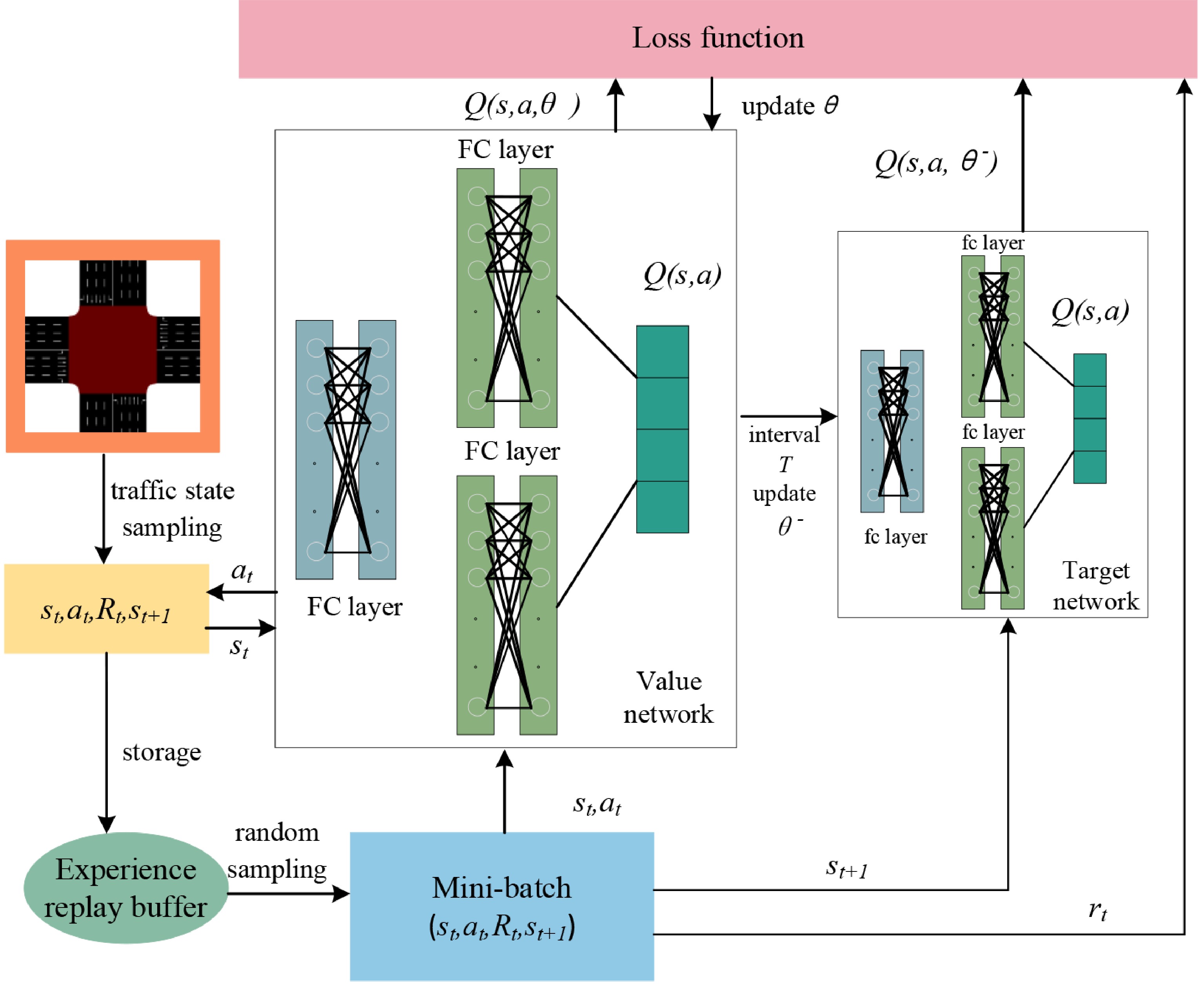
Figure 4.
Traffic signal control framework based on DDQN.
-
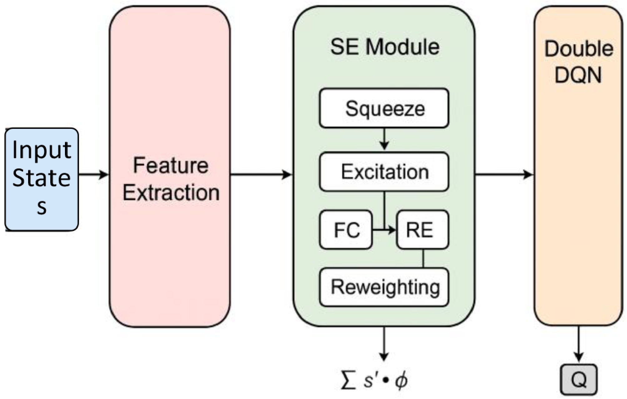
Figure 5.
Network architecture of the SE attention mechanism.
-
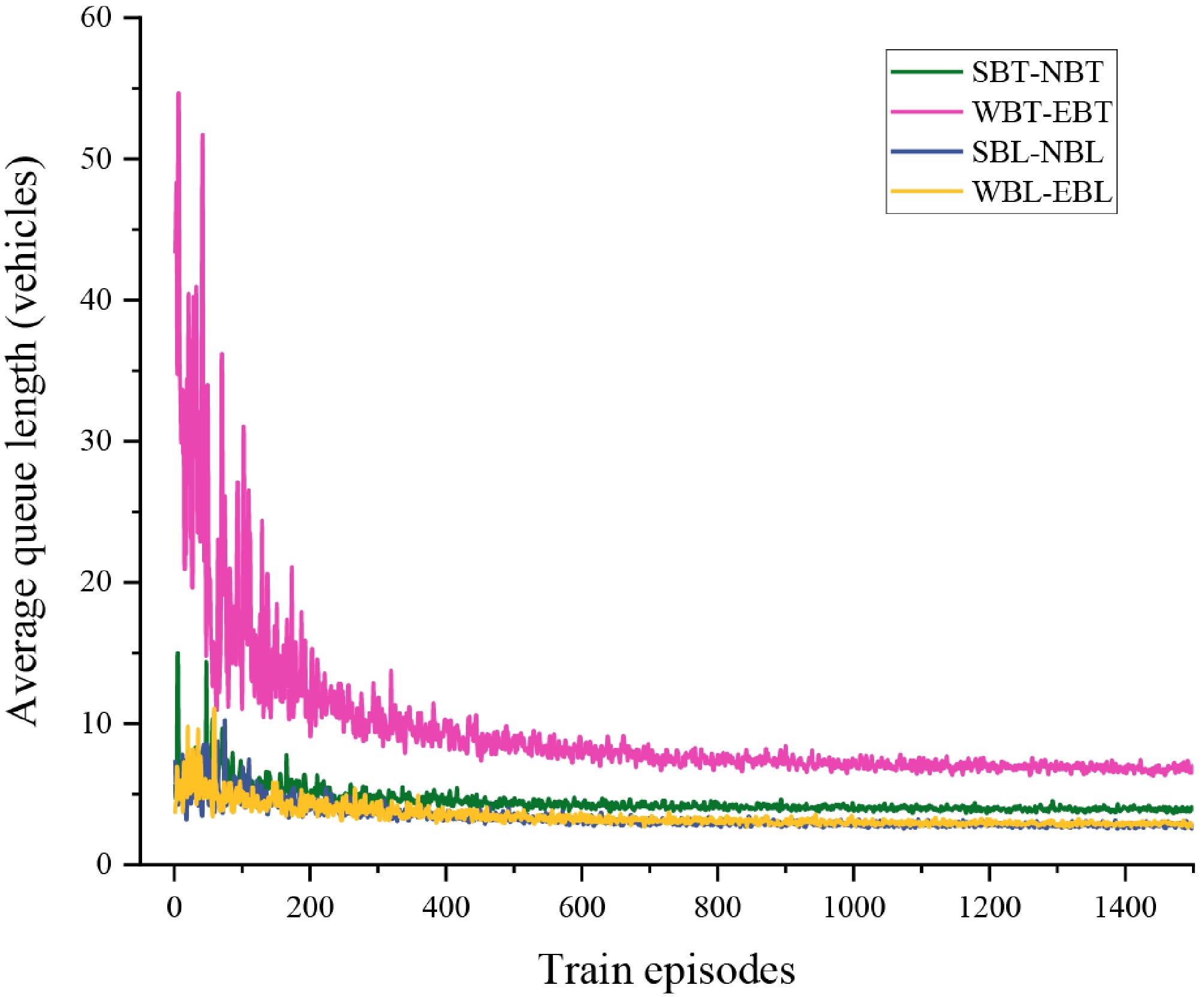
Figure 6.
The trend of average queue length variation for each traffic flow direction.
-
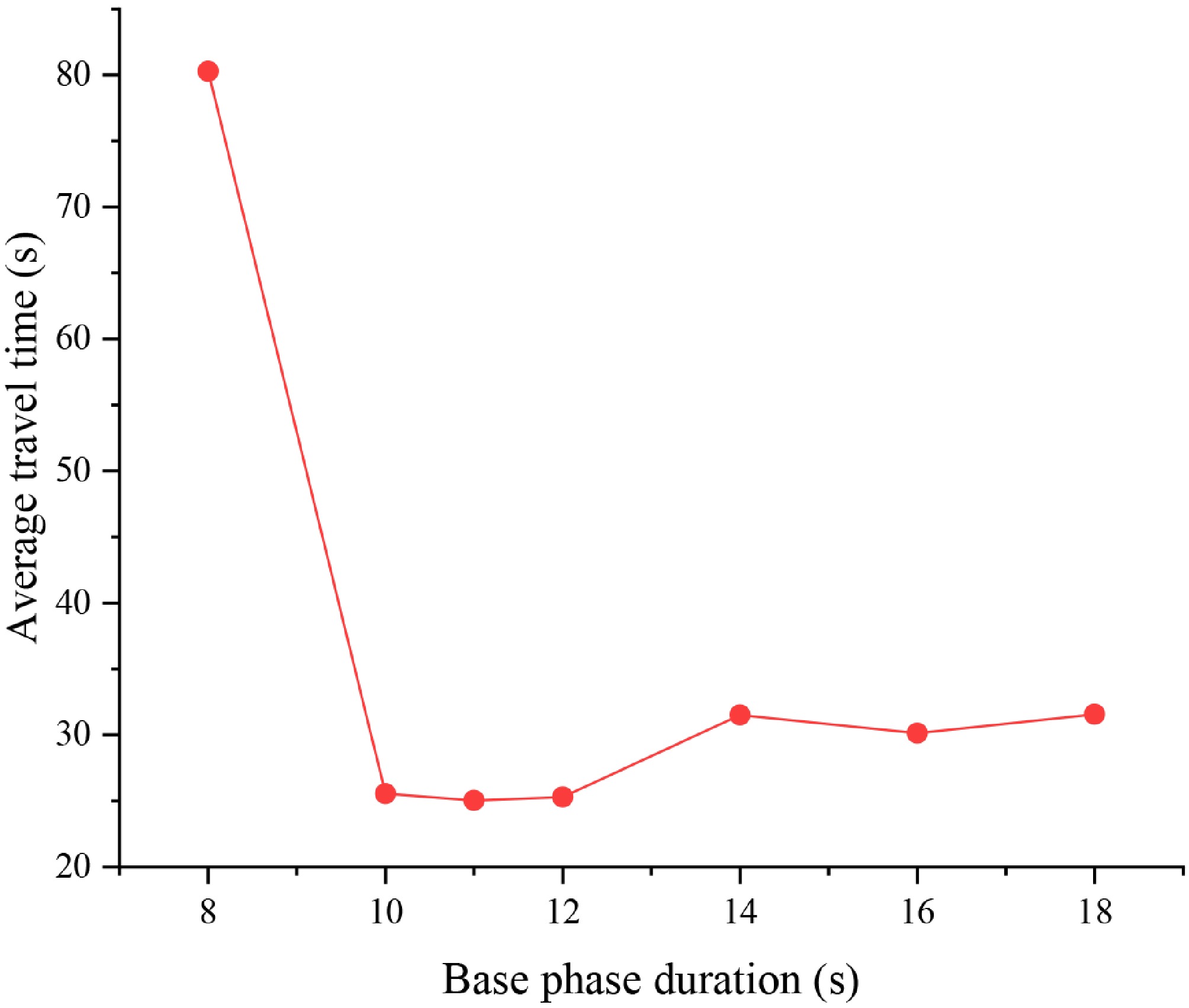
Figure 7.
Impact of base phase duration on the average travel time at the intersection.
-
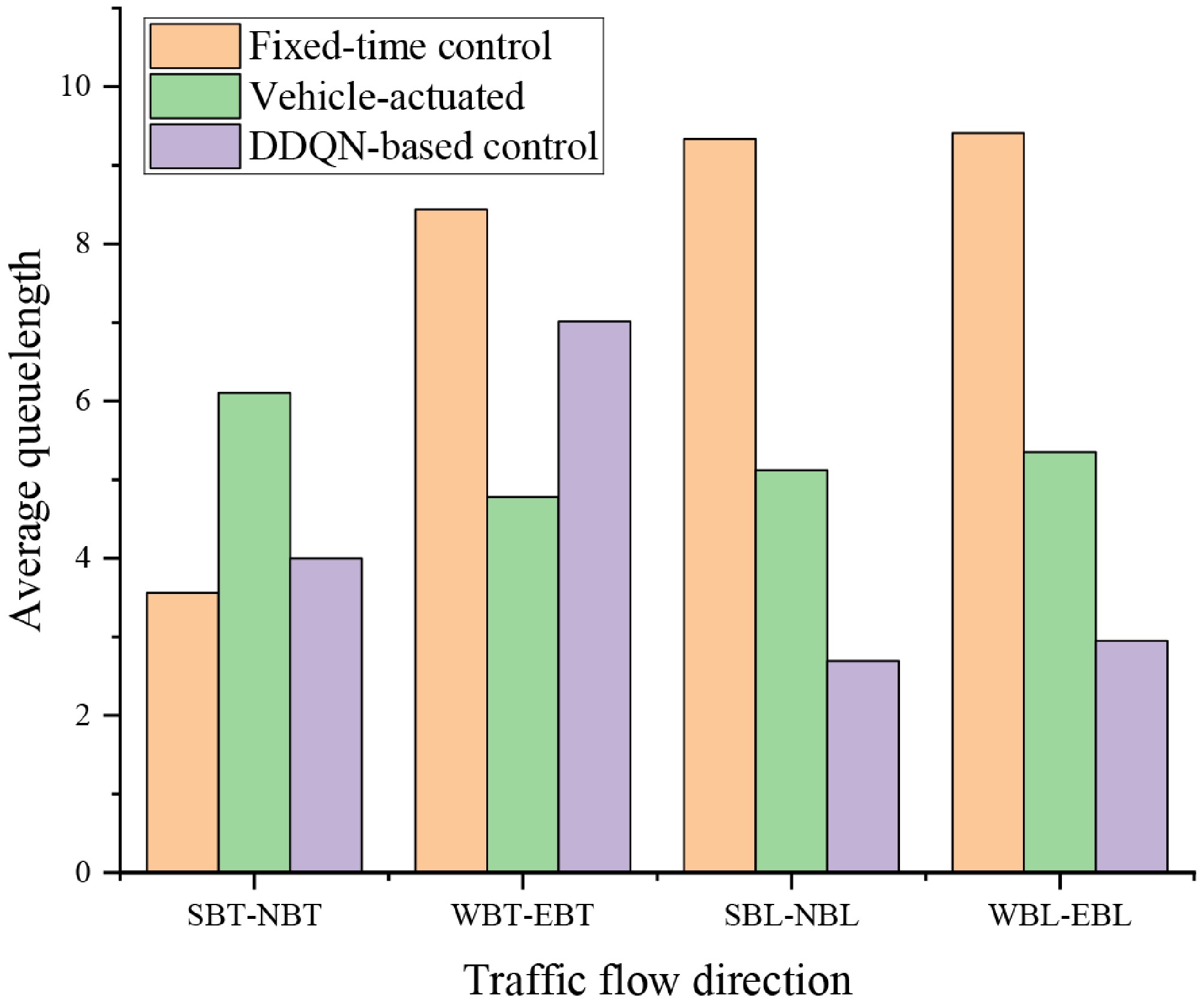
Figure 8.
Comparison of directional average queue lengths under three traffic signal control strategies.
-
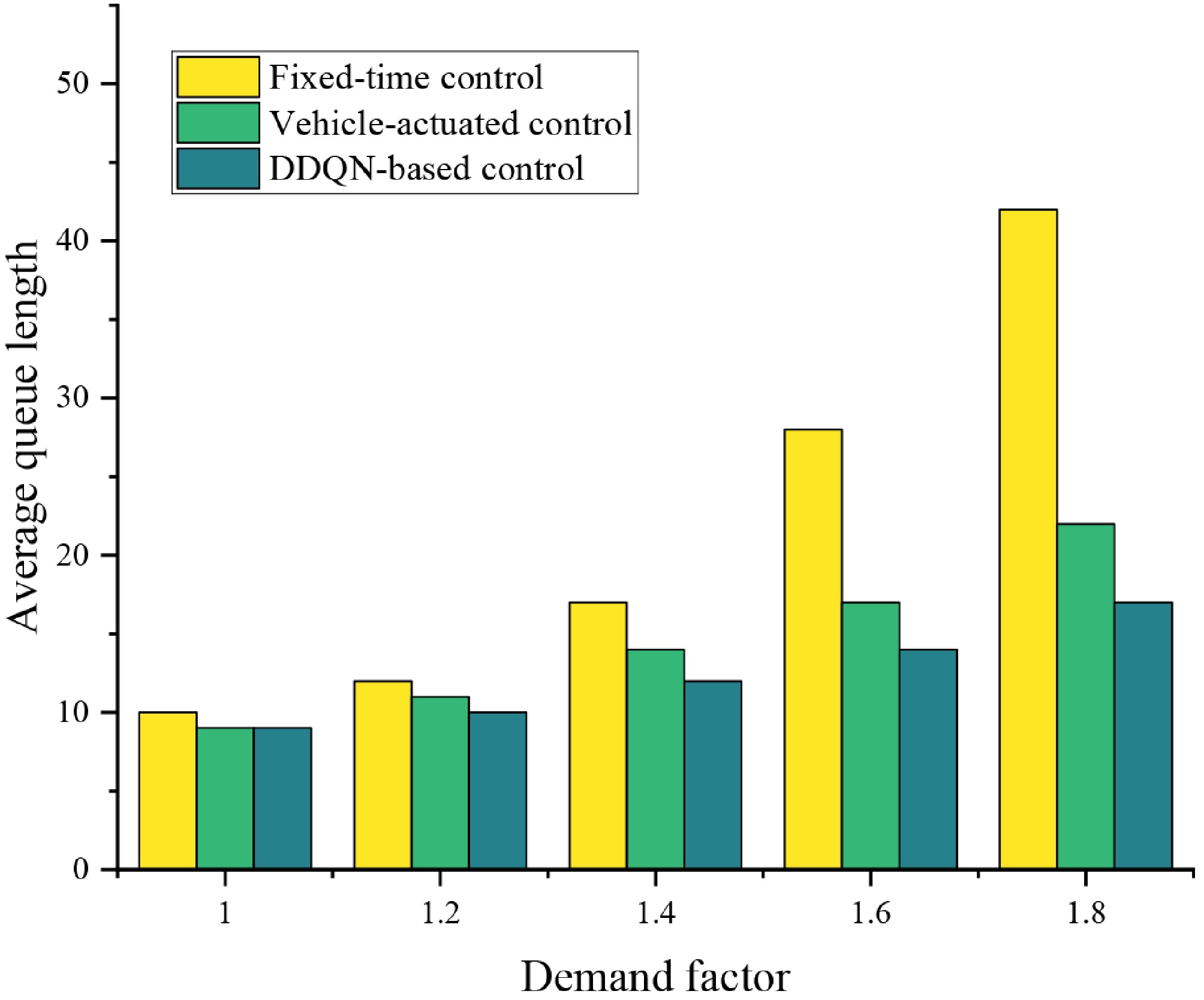
Figure 9.
Average queue length at the intersection under different demand levels.
-
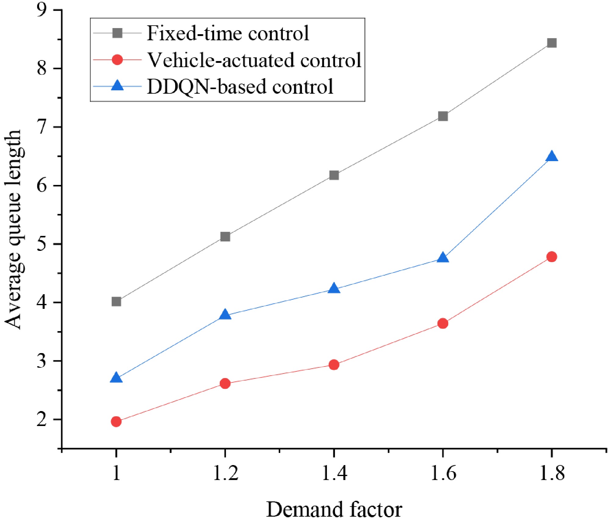
Figure 10.
Average queue length in the WBT-EBT direction under different demand levels.
-
Input: Discount factor γ; Learning rate α; Number of update iterations I; Target network update interval κ; Mini-batch size b; Number of training episodes N; Number of simulation steps T.
Output: Optimized network weights θ*.Initialization:
Initialize value network$ Q(\cdot ;\theta ) $ $ Q(\cdot ;{\theta }^{-}) $ $ {\theta }^{-}\leftarrow \theta $
Initialize experience replay buffer D;
Initialize update counter$ Counter\leftarrow 0 $ Detailed algorithm flow:
For episode n = 1 to N:Observe initial environment state s0 and take initial action a0;
For t = 1, 2, …, T:Observe current state st, and select action at based on ε-greedy policy;
Execute action at, observe next state st+1, and receive reward Rt;
Compute TD value:$ TD=y_{t}^{DDQN}-{Q}_{t}\left({s}_{t},{a}_{t};{\theta }_{t}\right) $
Store experience tuple$ \left\langle {\delta }_{t+1},({s}_{t},{a}_{t},{R}_{t},{s}_{t+1})\right\rangle $ End for If $ n\geq 2 $ For i = 1 to I: Sample a mini-batch B of size b from D;
Compute TD target yt using Eq. (6) with the target network;
Update θ by minimizing loss via gradient descent:$ \theta \leftarrow \theta -\alpha \nabla L(\theta ) $
Increment counter: Counter$ \leftarrow $ If Counter mod $ \kappa $ Update target network parameters: $ {\theta }^{-}\leftarrow \theta $ End if End for End if End for Table 1.
Signal control algorithm based on DDQN.
-
Entry approach Through (pcu/h) Left-turn (pcu/h) Westbound approach 400 100 Northbound approach 200 100 Eastbound approach 380 180 Southbound approach 200 150 Table 2.
Basic traffic demand.
-
Parameters Value Description Total training episodes 1,500 Total number of training episodes during which the agent interacts with the environment
and updates its policyMaximum simulation steps per episode 3,600 The maximum number of simulation steps executed in a single training episode Target network update interval κ 3 The target network is updated once every three updates of the main (evaluation) network Batch size 64 The number of samples used in each training batch for network parameter updates Learning rate α 0.0025 The learning rate used for training the DDQN network Discount factor γ 0.95 The discount factor used to calculate the cumulative future reward Table 3.
Value used for training parameters.
-
Traffic movement Fixed-time control Vehicle-actuated control DDQN-based control SBT-NBT 21.63 37.06 24.29 WBT-EBT 51.26 29.03 42.60 SBL-NBL 56.71 32.10 16.36 WBL-EBL 57.16 32.49 17.91 The bold value represents the minimum value, indicating that under the corresponding control method, this traffic flow direction has the best control traffic efficiency. Table 4.
Average travel time under the three control strategies.
Figures
(10)
Tables
(4)