-
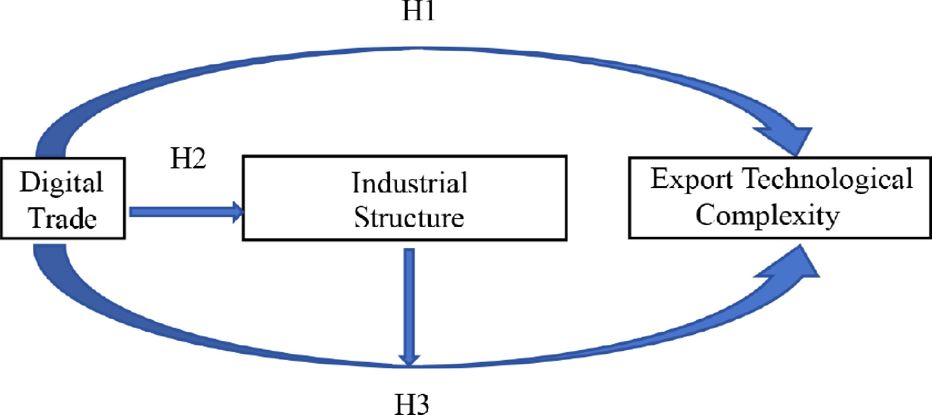
Figure 1.
Theoretical model of this paper.
-
Primary indicator Secondary indicator Tertiary indicator Code Digital trade infrastructure Information network infrastructure Length of long-haul fiber-optic cables (10,000 km) X1 Number of internet broadband access ports (10,000) X2 Population penetration rate of mobile phones (%) X3 Logistics transport infrastructure Number of operational freight trucks on highways (10,000) X4 Number of civil transport ships/units X5 Express delivery volume/million items X6 Digital technological innovation Technological innovation input Number of patents granted (1,000) X7 R & D expenditure/10 billion RMB X8 Digital innovation output Technology market transaction volume (billion RMB) X9 Digital trade market Digital supply Total telecommunications services volume (100 billion RMB) X10 Total postal services volume/billion RMB X11 Digital demand Software services revenue (billion RMB) X12 E-commerce sales volume/billion RMB X13 Trade potential Economic strength GDP (100 million RMB) X14 Trade scale Total import and export trade volume ( ${\text{\$}} $ X15 Source: compiled by the author. Table 1.
Digital trade measurement indicators.
-
Index Variable name (Abbreviation) Calculation formula 1 Economic development level (LNPgdp) LNPgdp Logarithm of GDP per capita 2 Human capital level (HC) Number of students in higher education/Total population 3 Industrialization level (IL) Industrial value added/Gross regional product 4 Openness degree (OPEN) Total import and export trade volume/GDP 5 Social consumption level (SCL) Total retail sales of consumer goods/Gross regional product Source: compiled by the author. Table 2.
Control variables.
-
VIF 1/VIF Dtra 3.131 0.319 HC 1.535 0.651 IND 4.305 0.232 IL 2.562 0.390 LNPgdp 4.482 0.223 OPEN 1.893 0.528 SCL 1.478 0.676 Mean VIF 2.770 Source: compiled by the author. Table 3.
Multicollinearity test.
-
(1) Expy (2) Expy (3) Expy (4) Expy (5) Expy (6) Expy Dtra 2.209*** 1.471*** 0.702*** 0.735*** 0.767*** 0.704*** (39.796) (21.551) (7.745) (8.119) (8.505) (7.806) HC 0.663*** 0.387*** 0.381*** 0.346*** 0.405*** (14.235) (8.210) (8.145) (7.271) (8.188) LNPgdp 0.790*** 0.777*** 0.810*** 0.768*** (11.171) (11.067) (11.519) (10.974) SCL −0.079*** −0.058** −0.045 (−2.799) (−2.013) (−1.600) IL 0.113*** 0.131*** (2.978) (3.475) OPEN −0.229*** (−3.673) Observations 390 390 390 390 390 390 R2 0.815 0.882 0.913 0.914 0.917 0.920 F 1583.7 1337.9 1242.0 951.3 779.6 674.8 *, **, *** indicates significant at the significance level of 10%, 5%, and 1% respectively, the content inside () represents the t-statistic. Table 4.
Basic regression results.
-
(1) Expy (2) Expy (3) Expy (4) Expy Dtra 0.294*** 1.074*** 0.649*** (5.011) (10.012) (6.576) DT 0.651*** (6.803) HC 0.241*** 0.371*** 0.352*** 0.471*** (5.623) (6.357) (7.095) (8.312) LNPgdp 0.660*** 0.646*** 0.704*** 0.928*** (10.607) (7.994) (10.789) (11.928) SCL −0.077** −0.019 −0.050* −0.060* (−2.022) (−0.635) (−1.707) (−1.825) IL −0.098*** 0.121*** 0.094** 0.204*** (−2.727) (2.728) (2.485) (4.518) OPEN −0.682*** −0.283*** −0.203*** −0.227*** (−14.743) (−3.959) (−3.131) (−2.904) N 360 300 338 390 R2 0.927 0.916 0.917 F 558.7 559.6 648.9 *, **, and *** respectively indicate significant at the significance level of 10%, 5%, and 1%, the content inside () represents the t-statistic. Table 5.
Results of robustness tests.
-
(1) IND (2) Expy Dtra 0.692*** 0.473*** (7.300) (5.209) IND 0.335*** (7.063) HC 0.175*** 0.346*** (3.372) (7.352) LNPgdp 0.001 0.768*** (0.007) (11.705) SCL 0.112*** −0.083*** (3.769) (−3.061) IL −0.468*** 0.288*** (−11.827) (6.898) OPEN 0.010 −0.233*** (0.160) (−3.979) N 390 390 R2 0.730 0.930 F 159.1 665.4 *, **, *** indicates significant at the significance level of 10%, 5%, and 1% respectively, the content inside () represents the t-statistic. Table 6.
Regression results of mediating effects.
-
Region Specific province Coastal cities Liaoning Province, Hebei Province, Beijing Municipality, Tianjin Municipality, Shandong Province, Jiangsu Province, Shanghai Municipality, Zhejiang Province, Fujian Province, Guangdong Province, Guangxi Zhuang Autonomous Region, Hainan Province Inland cities Shanxi Province, Jilin Province, Heilongjiang Province, Anhui Province, Jiangxi Province, Henan Province, Hubei Province, Hunan Province, Sichuan Province, Guizhou Province, Yunnan Province, Shaanxi Province, Gansu Province, Qinghai Province, Inner Mongolia Autonomous Region, Ningxia Hui Autonomous Region, Chongqing Municipality Data source: Compiled based on the documents of the National Development, and Reform Commission and the National Bureau of Statistics of China. Table 7.
Regional division.
-
Coastal cities expy Inland cities expy Dtra 0.941*** 0.280*** (6.353) (3.172) HC 0.440*** 0.389*** (5.634) (6.365) LNPgdp 0.774*** 0.720*** (6.539) (11.079) SCL 0.030 −0.031 (0.672) (−0.876) LI 0.166* 0.080*** (1.746) (2.767) OPEN −0.071 −0.056 (−0.817) (−1.400) N 156 234 R2 0.925 0.932 F 285.7 477.2 *, **, *** indicates significant at the significance level of 10%, 5%, and 1% respectively, the content inside () represents the t-statistic. Table 8.
Regional heterogeneity regression results.
Figures
(1)
Tables
(8)