-
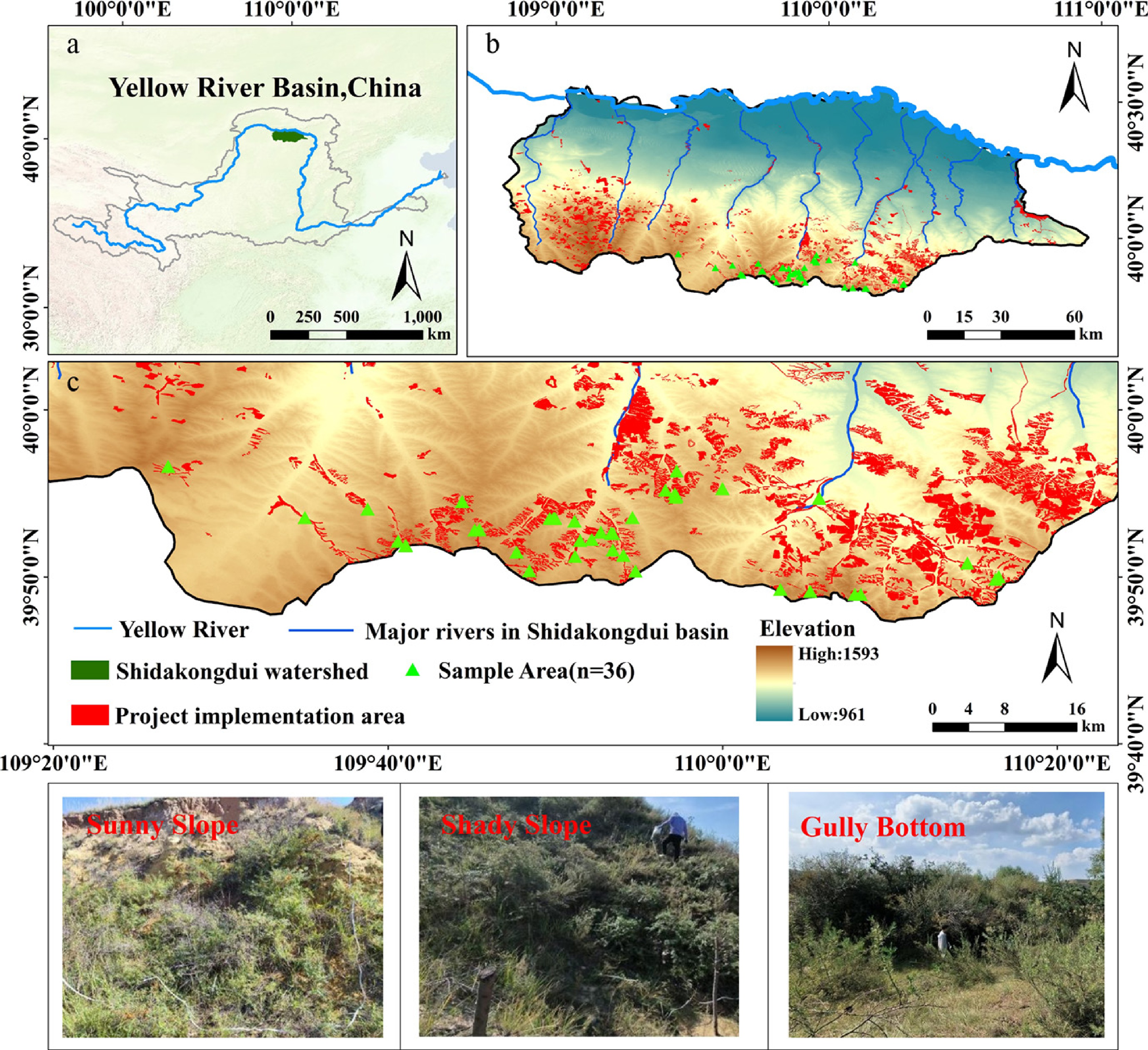
Figure 1.
Study area and sample plot distribution. (a) Geographical location of the Shidakongdui Basin in the Yellow River Basin; (b) Topography, river system and distribution of ecological restoration projects; (c) Detailed distribution of sampling sites and project implementation areas. Data sources: the digital elevation model (DEM) was derived from the ALOS World 3D (AW3D) 12.5 m dataset (Japan Aerospace Exploration Agency, JAXA,
https://nasadaacs.eos.nasa.gov/ ); the administrative boundary and river network data were obtained from the Resource and Environment Science and Data Center (RESDC), Chinese Academy of Sciences (https://resdc.cn/ ). -
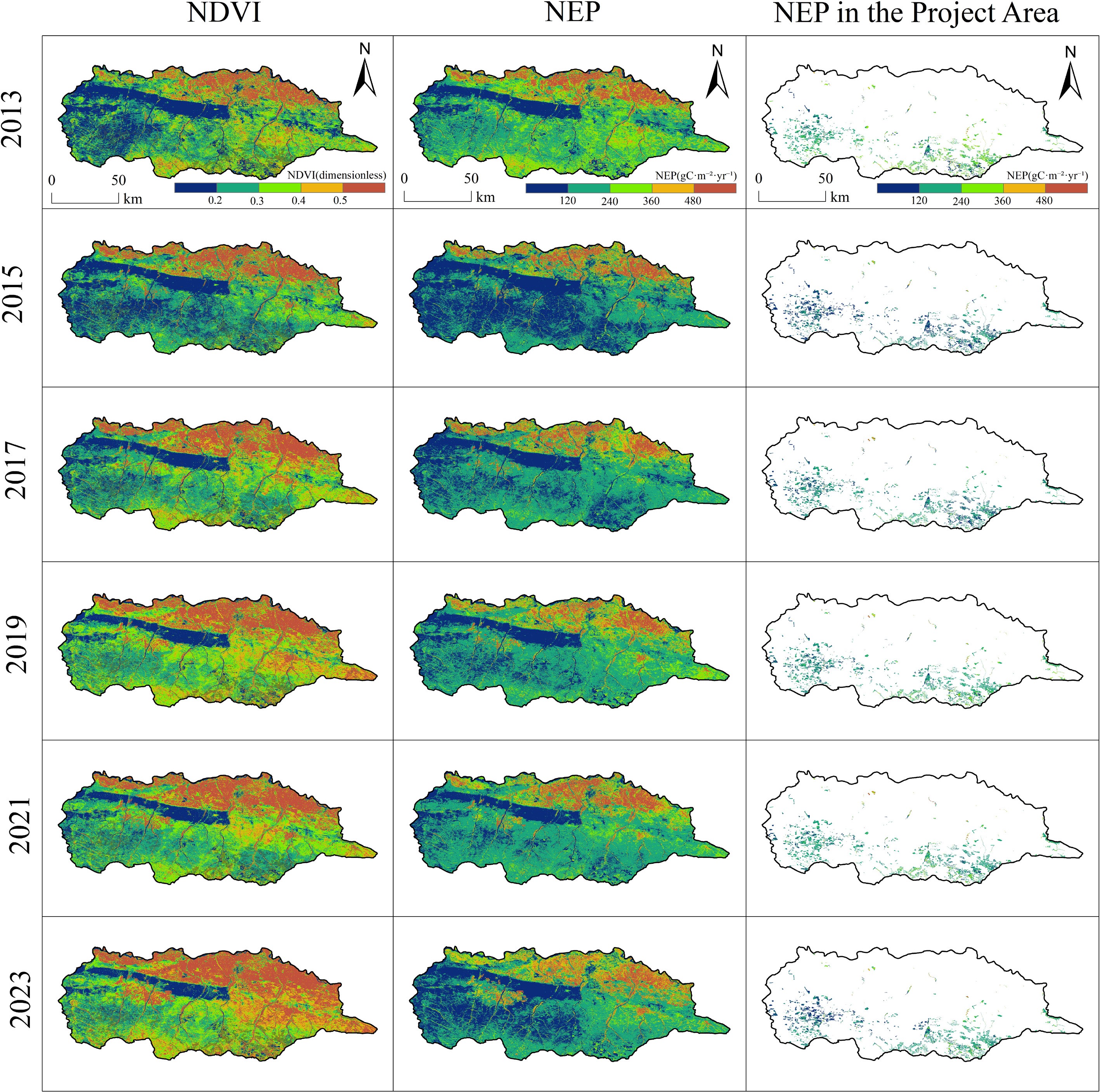
Figure 2.
Spatial distribution patterns of NDVI, NPP, and NEP in the study area, 2013–2023.
-
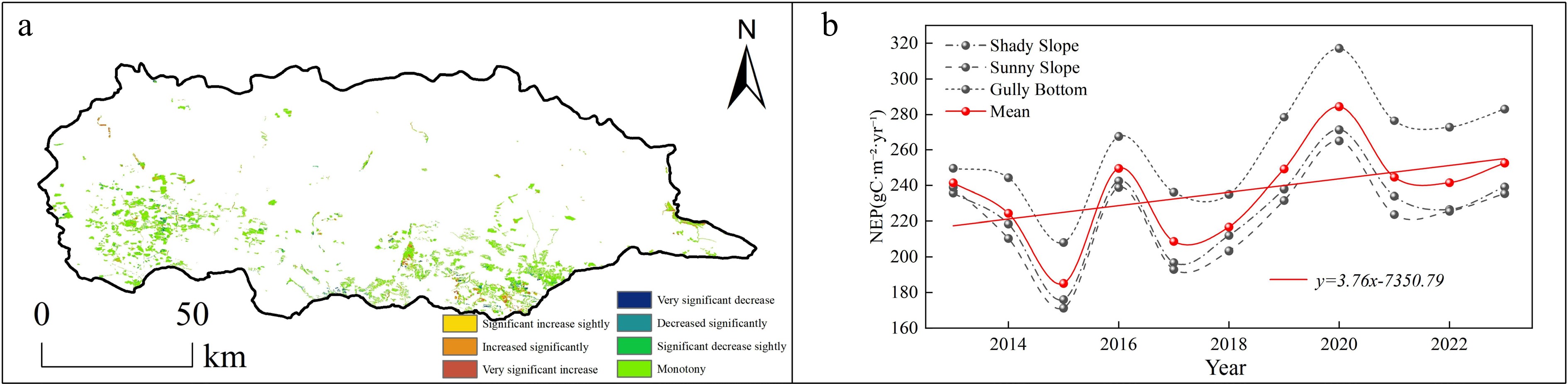
Figure 3.
Spatio-temporal variation trends of NEP in the study area. (a) Spatial distribution of NEP change trends in Hippophae rhamnoides L. plantation stands 2013–2023; (b) temporal variation trend of NEP in Hippophae rhamnoides L. plantation stands 2013–2023.
-
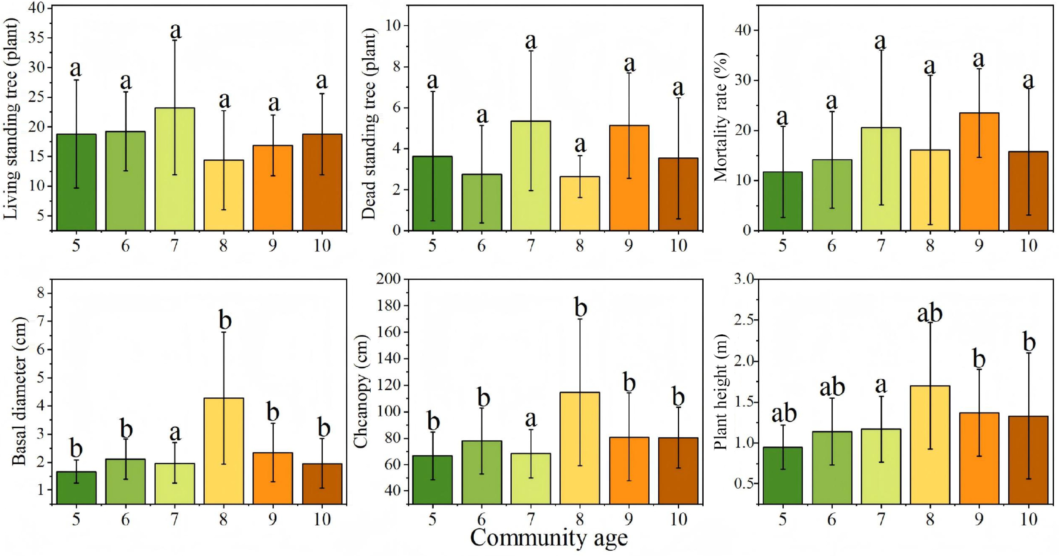
Figure 4.
Growth characteristics of Hippophae rhamnoides L. plantation stands across different stand ages. n = 36 sample plots.
-
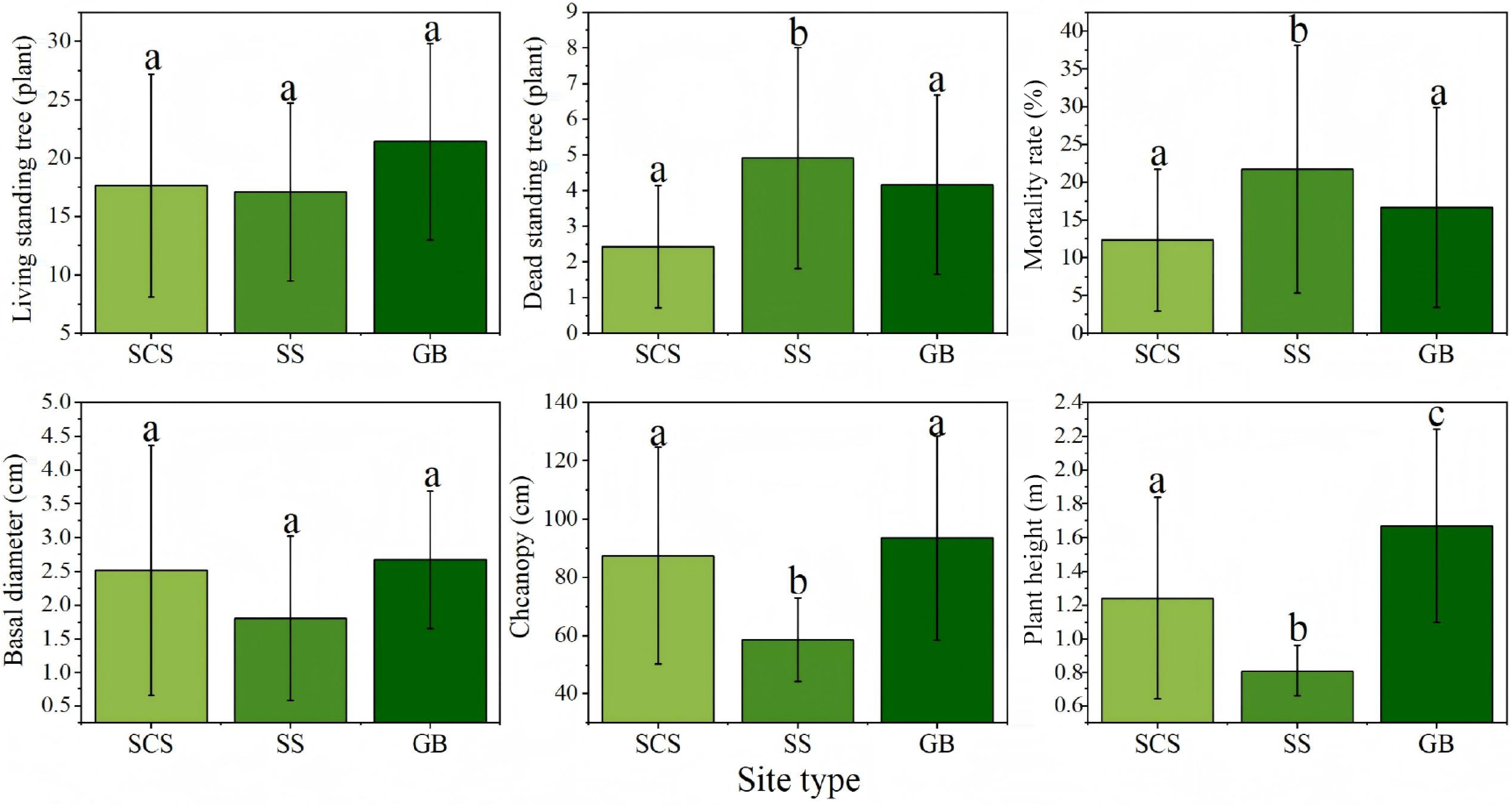
Figure 5.
Growth characteristics of Hippophae rhamnoides L. plantation stands across different site types. n = 36 sample plots. SCS: shady slope; SS: sunny slope; GB: gully bottom.
-

Figure 6.
Optimal single- and dual-factor growth models for Hippophae rhamnoides L. n = 36 sample plots. (a) Single-factor growth model of above-ground biomass; (b) Single-factor growth model of below-ground biomass; (c) Dual-factor growth model of above-ground biomass; (d) Dual-factor growth model of below-ground biomass.
-
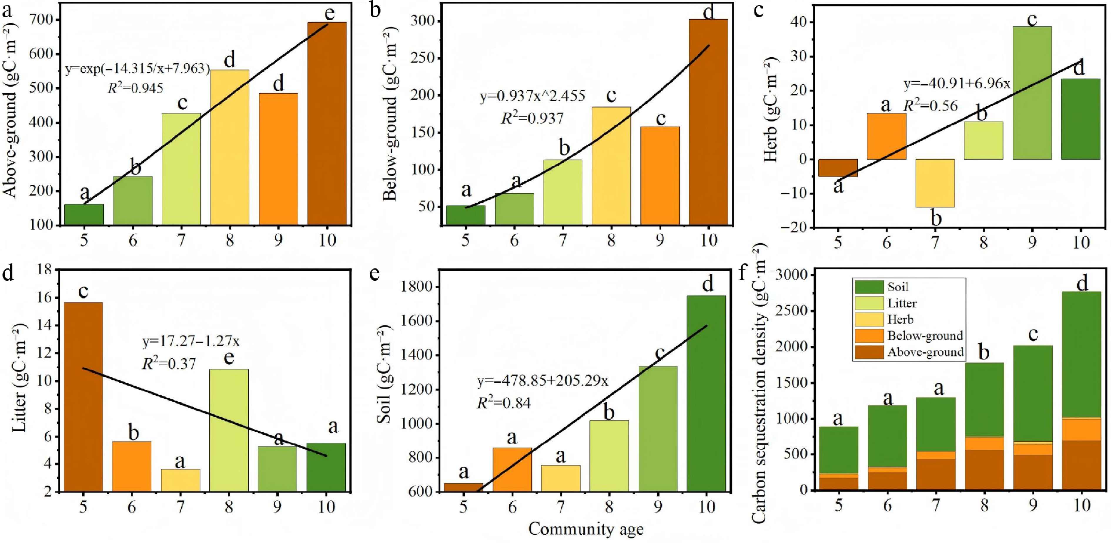
Figure 7.
Distribution of carbon sequestration density in Hippophae rhamnoides L. plantation stands 2013–2018. (a) Above-ground carbon sequestration density; (b) below-ground carbon sequestration density; (c) herb layer carbon sequestration density; (d) litter layer carbon sequestration density; (e) soil carbon sequestration density, and (f) total ecosystem carbon sequestration density.
-
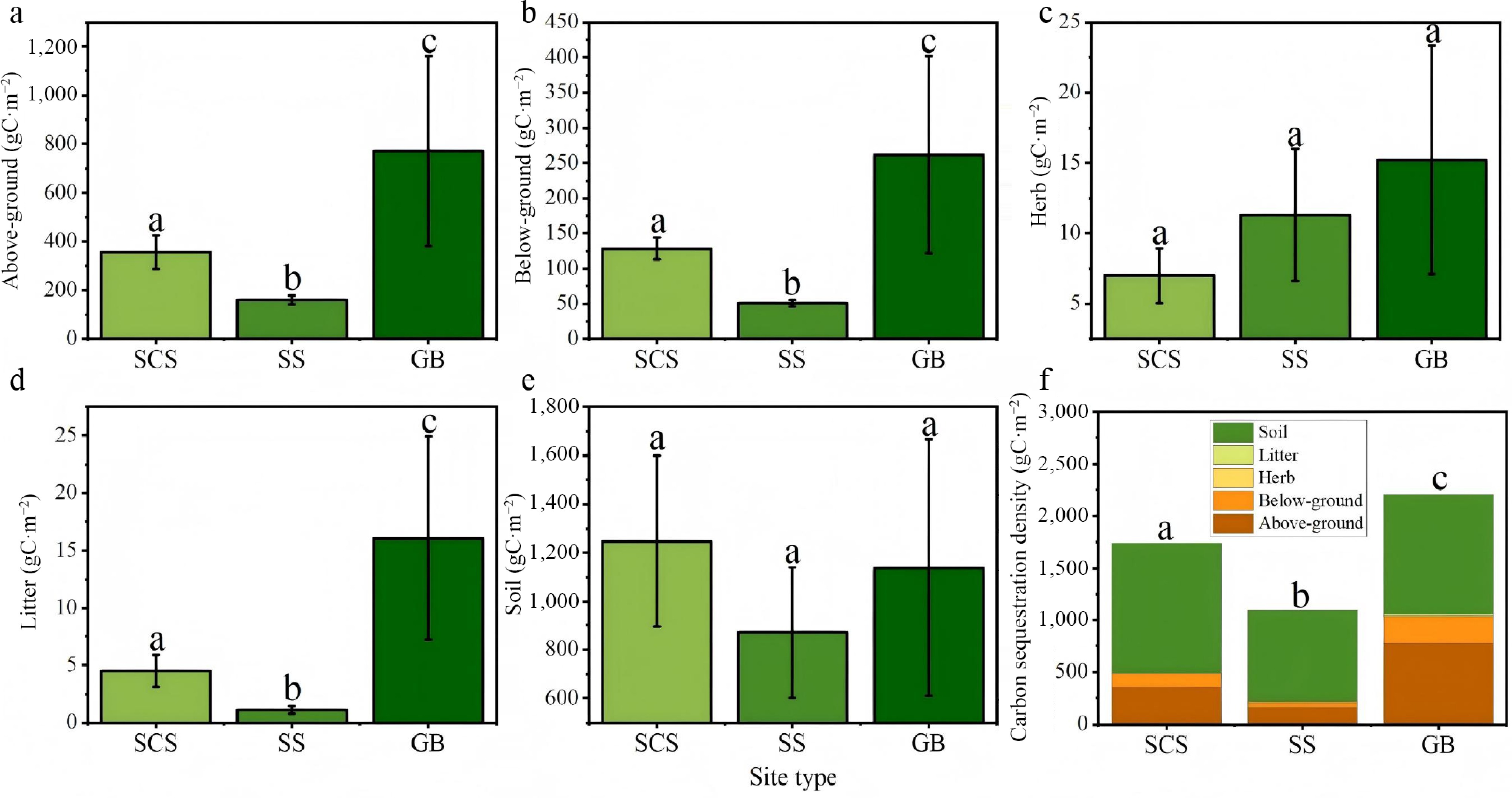
Figure 8.
Carbon sequestration density of Hippophae rhamnoides L. plantation stands across different site types. (a) Above-ground carbon sequestration density; (b) below-ground carbon sequestration density; (c) herb layer carbon sequestration density; (d) litter layer carbon sequestration density; (e) soil carbon sequestration density, and (f) total ecosystem carbon sequestration density. SCS: shady slope; SS: sunny slope; GB: gully bottom.
-
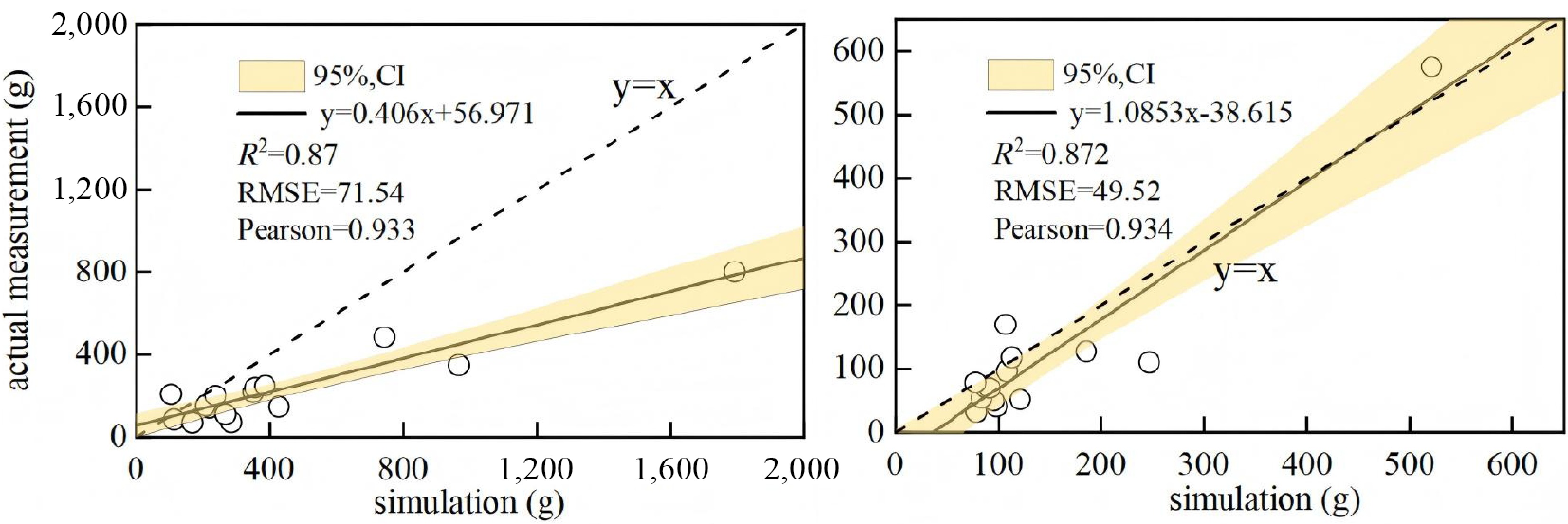
Figure 9.
Goodness-of-fit validation for the Hippophae rhamnoides L. growth model.
-
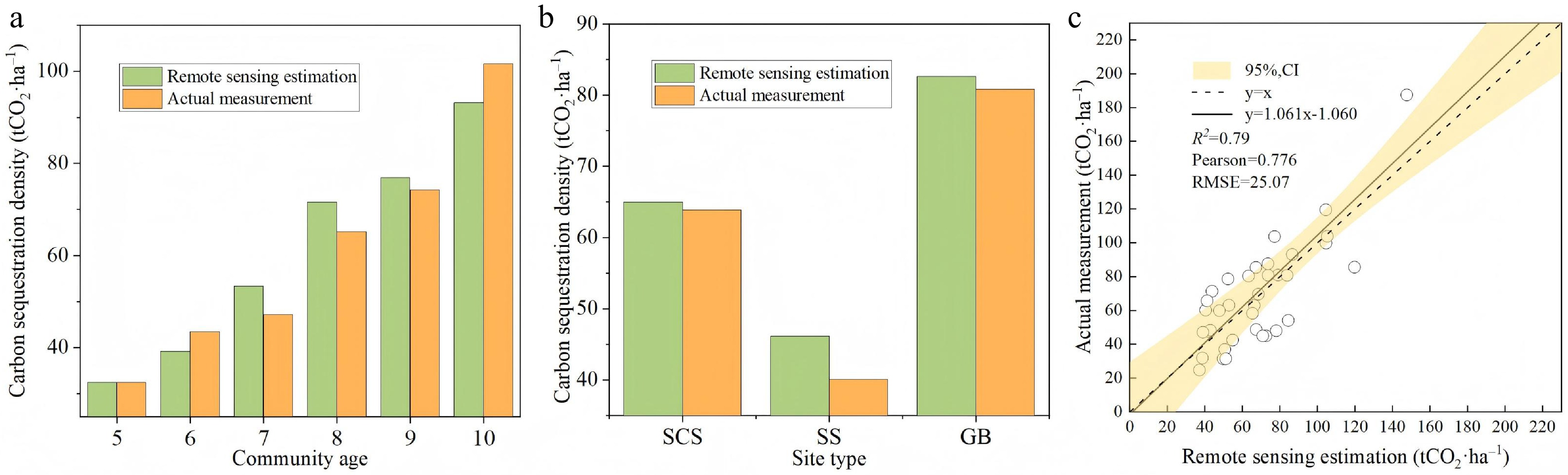
Figure 10.
Goodness-of-Fit Between Remote Sensing-Derived and Field-Measured Carbon Sequestration Density in Hippophae rhamnoides L. Plantation Stands. (a) Comparison of remote sensing-derived and field-measured carbon sequestration density across different stand ages; (b) comparison of remote sensing-derived and field-measured carbon sequestration density across different site types; (c) comparison of remote sensing-derived and field-measured carbon sequestration density across all 36 sample plots. SCS: shady slope; SS: sunny slope; GB: gully bottom.
-
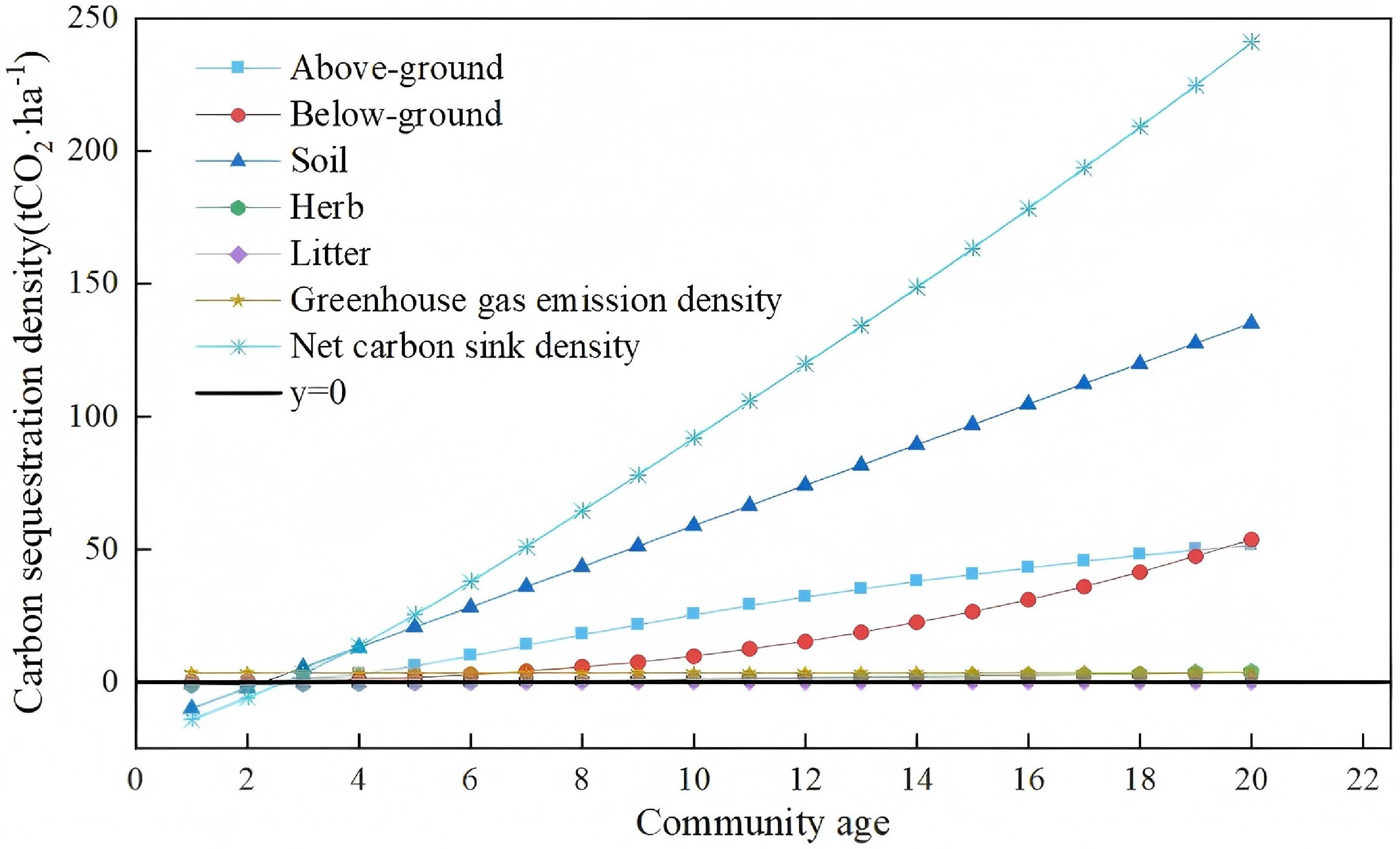
Figure 11.
Year-by-year prediction of carbon sequestration density for Hippophae rhamnoides L. plantation stands in the study area.
-
Data classes Products Temporal resolution Spatial resolution Landsat 8 OLI LANDSAT/LC08/C02/T1_L2 16 d 30 m Landsat 7 ETM+ LANDSAT/LE07/C02/T1_L2 2008–2013 30 m Meteorological data ECMWF ERAS-Land 30 d 11,132 m DEM ALOS Static 12.5 m NDVI LANDSAT/LC08/C02/T1_L2 16 d 30 m Table 1.
Data sources.
-
Community age (years) Herb cover (%) Stand density
(plant·ha−1)Sample plots Experimental plots Control plots Herbaceous and
litter subplotsSoil sampling
points10 52−88 2,400−11,600 7 14 7 42 28 9 65−75 7,200−10,800 4 8 4 24 16 8 55−85 2,800−11,600 6 12 6 36 24 7 36−86 5,200−15,600 7 14 7 42 28 6 60−92 7,200−10,800 6 12 6 36 24 5 58−69 7,600−10,000 6 12 6 36 24 Table 2.
Sample information for Hippophae rhamnoides L. plantation stand community surveys.
-
Soil depth Soil index Unit Community age 10 9 8 7 6 5 0−10 cm BD g/cm3 1.25 ± 0.17a 1.24 ± 0.24a 1.27 ± 0.14a 1.21 ± 0.35a 1.26 ± 0.21a 1.18 ± 0.21a SOC g/kg 6.2 ± 2.79a 4.44 ± 2.79b 3.48 ± 1.52b 3.12 ± 1.39b 3.76 ± 2.13b 3.04 ± 1.62b 10−20 cm BD g/cm3 1.29 ± 0.18a 1.26 ± 0.29a 1.42 ± 0.59a 1.26 ± 0.24a 1.24 ± 0.15a 1.26 ± 0.15a SOC g/kg 4.49 ± 2.07a 3.37 ± 1.96ab 2.56 ± 1.18bc 1.92 ± 0.31c 2.22 ± 1.11bc 2.3 ± 0.91bc 20−50 cm BD g/cm3 1.25 ± 0.11a 1.16 ± 0.27a 1.31 ± 0.16a 1.16 ± 0.34a 1.28 ± 0.15a 1.24 ± 0.14a SOC g/kg 4.46 ± 2.53a 4.52 ± 3.36a 2.69 ± 2.22b 2.08 ± 0.98b 2.06 ± 0.75b 2.06 ± 0.75b Table 3.
Soil characteristics of Hippophae rhamnoides L. plantation stands across different stand ages.
-
Model R2 Single-factor Above-ground biomass Wt = −0.503H + 0.526H2 + 0.021H3 + 0.194 0.871 Below-ground biomass Wd = 0.934H − 0.772H2 + 0.233H3 − 0.286 0.892 Dual-factor Above-ground biomass Wt = 0.228D^0.1 × H^2.488 + 0.006 0.923 Below-ground biomass Wd = 0.018D^0.1 × H^3.981 + 0.073 0.898 Where Wt and Wd represent above-ground and below-ground biomass (kg), respectively; D is the ground diameter (cm); and H denotes plant height (m). Table 4.
Optimal single- and dual-factor growth models for Hippophae rhamnoides L.
Figures
(11)
Tables
(4)