Back Article

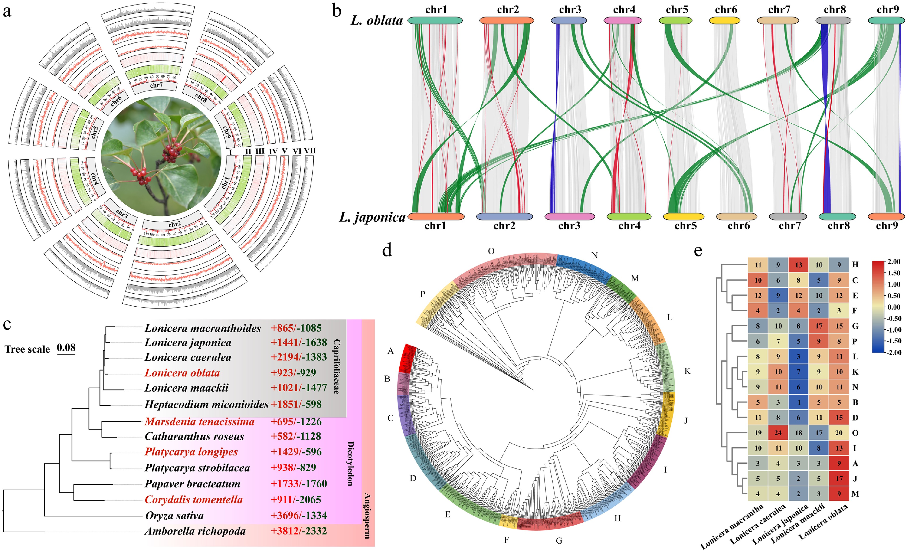
Figure 1. 

Genome assembly and comparative genomic analyses of Lonicera oblata. (a) Genomic characterization of L. oblata; (I) Chromosome, (II) Gene density, (III) GC content, (IV) Long terminal repeat retrotransposons (LTRs) content, (V) LTR-Gypsy content, (VI) LTR-Copia content, (VII) DNA transposons. (b) Collinearity analysis between L. oblata and L. japonica. The gray segments represent the gene collinearity, the blue segments represent chromosomal inversions, and the orange and red segments represent chromosomal translocations. (c) Phylogenetic tree of 14 species reconstructed from 238 single-copy orthologs. The samples with red Latin names are limestone-endemic species. The red and green numbers on the right indicate the number of orthologous groups that have expanded and contracted, respectively, compared to closely related species. (d) Phylogenetic tree of the bHLH family from Lonicera, constructed using the maximum-likelihood method (JTT + R6 model; 1,000 bootstrap replicates). The colored bands divide the bHLH family into 16 subfamilies. (e) Heatmap of the bHLH subfamilies in Lonicera; the numbers in the heatmap represent the number of gene subfamilies for each corresponding species. The red-blue gradient illustrates the variability of the number of subfamily genes.

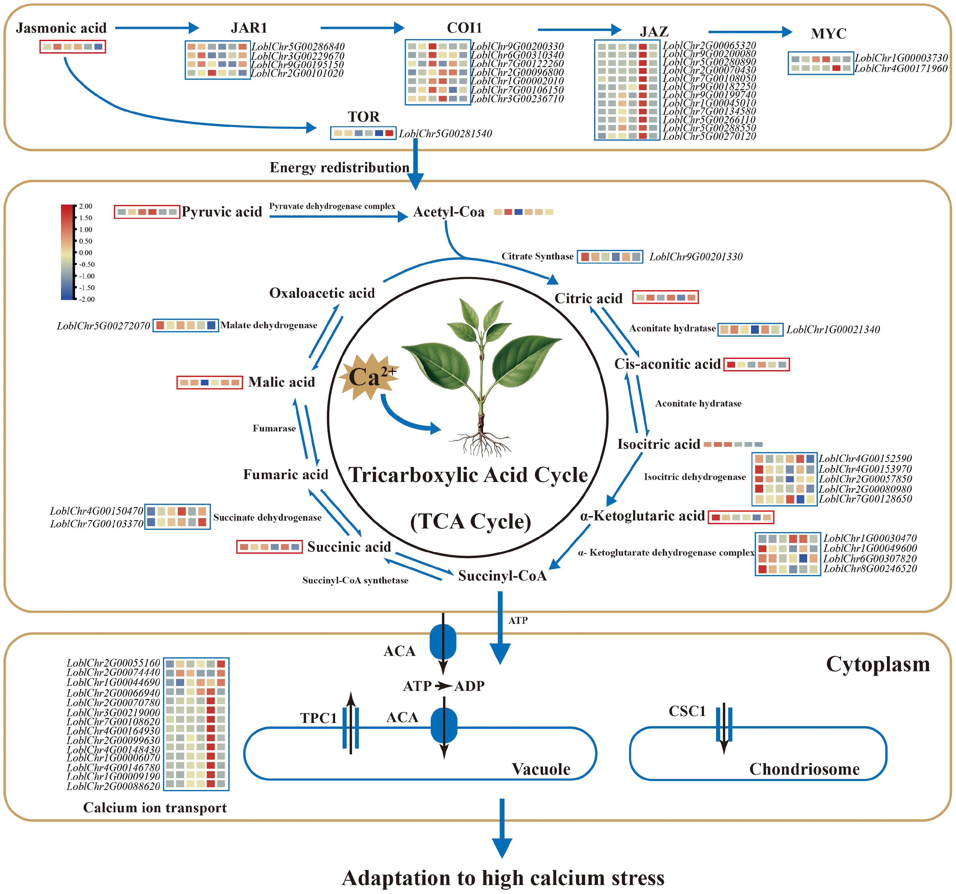
Figure 2. 

Mechanism of high Ca²⁺ adaptation in Lonicera oblata. The blue box represents the expression of the differentially expressed genes, while the red box reflects the abundance of differentially accumulated metabolites. The colored blocks within each box are arranged (left to right) in chronological order corresponding to the following time points: control (CK), 1, 3, 6, 12, and 24 h. Calcium stress induced pronounced changes in jasmonic acid (JA) signaling and TOR responses, with rapid induction of JAR1 (peaking at 1 h), overall upregulation of COI1, strong induction of multiple JAZ genes during early to mid-stages, and significant activation of MYC2/3 transcription factors, whereas TOR expression was reduced from 1 to 12 h. In the tricarboxylic acid (TCA) cycle, pyruvic acid increased from 1 h onward, citric acid accumulated at 1 and 6 h, while cis-aconitic acid and α-ketoglutaric acid decreased at early time points. Downstream intermediates, including succinic acid and malic acid, accumulated during 6–12 h and partially recovered by 24 h. The genes encoding aconitate hydratase and isocitrate dehydrogenase were differentially expressed at early stages, whereas fumarase, succinate dehydrogenase, and malate dehydrogenase genes showed higher expression at later stages. Most calcium ion transporter genes were differentially expressed, with expression levels peaking around 12 h. Calcium ion homeostasis under stress is achieved through JA-mediated organic acid chelation and active transport mechanisms.

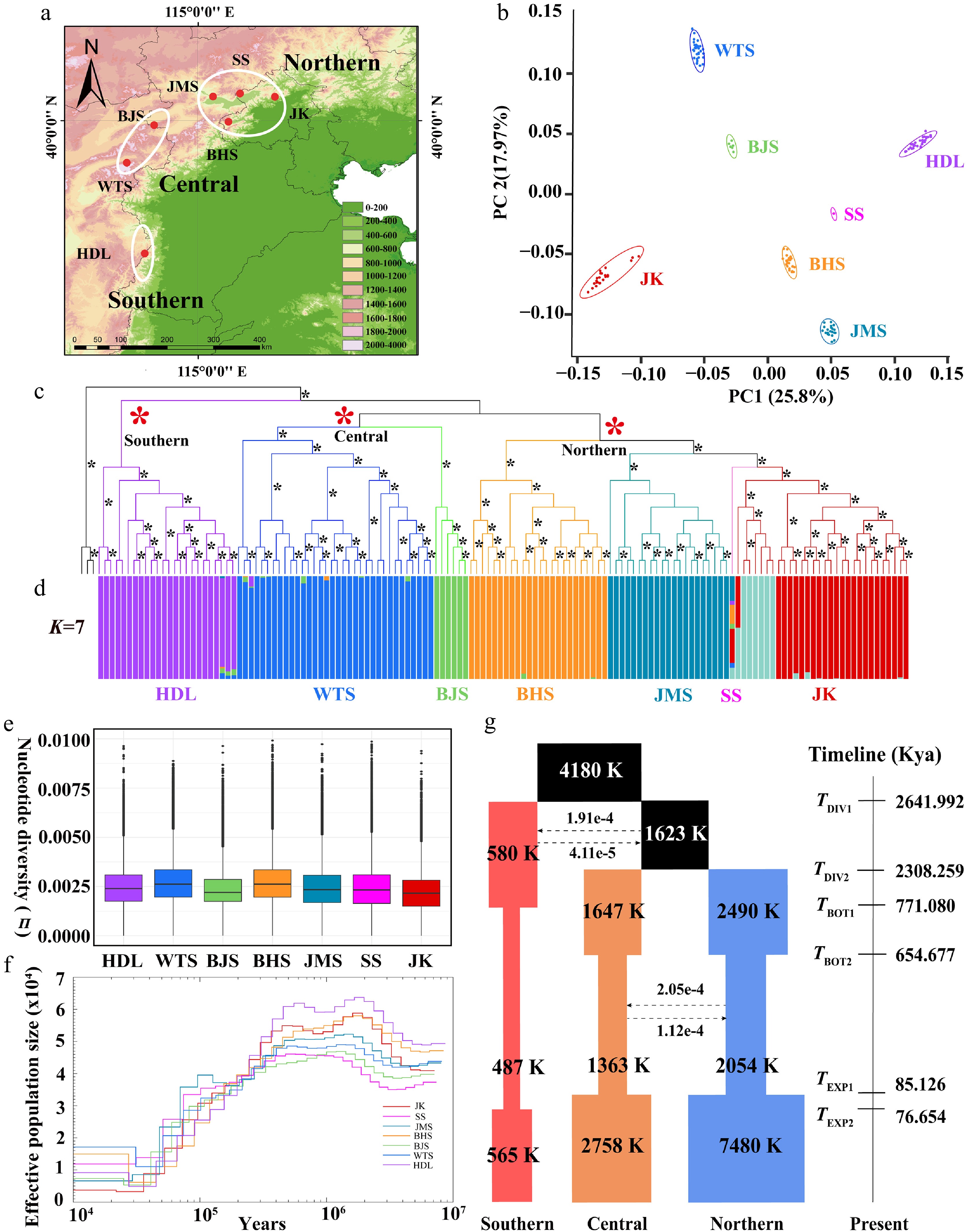
Figure 3. 

Distribution pattern, population structure, genetic diversity, and demographic history of Lonicera oblata. (a) Geographic distribution of the seven populations. (b) PCA plot of L. oblata populations. (c) A maximum likelihood phylogenetic tree of 140 L. oblata individuals, with L. webbiana as the outgroup; branches with full support (ultrafast bootstrap value = 100) are marked with *. (d) Population structure of L. oblata inferred by Admixture (optimal K = 7). (e) Nucleotide diversity (π) among the seven populations. (f) Pairwise Sequentially Markovian Coalescent (PSMC) modeling analysis of the seven populations of L. oblata, with a generation time of 10 years and a mutation rate (μ) of 1.43e–8 per site per generation. (g) Maximum likelihood estimation of the best-fit model (model 11) in fastsimcoal2 (see Supplementary Table S14). (a) The map is from the National Platform for Common Geospatial Information Services (Tianditu), with review number GS(2024)0650. Source: www.tianditu.gov.cn.

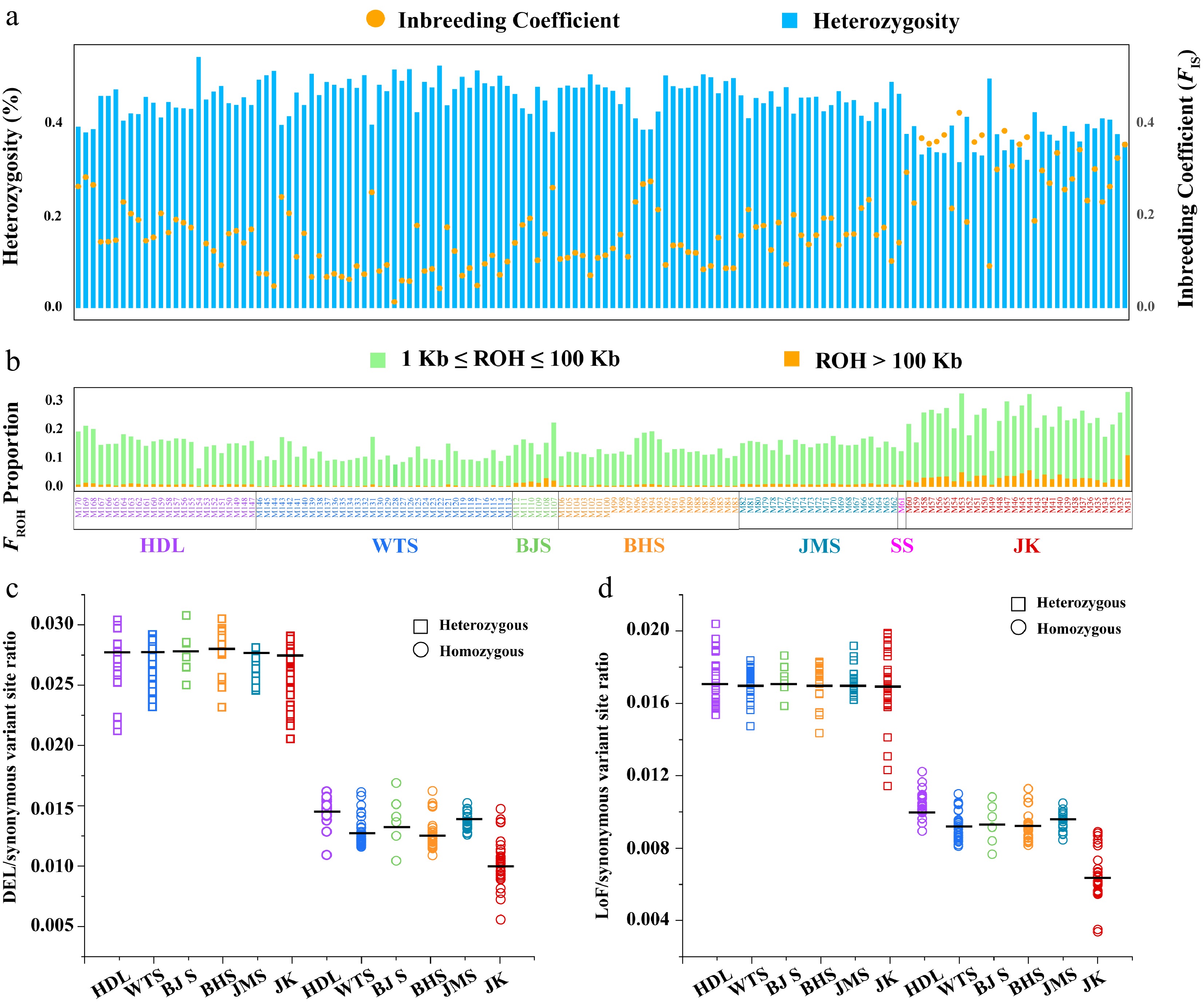
Figure 4. 

Analyses of inbreeding and genetic load. (a) Per-site genome-wide heterozygosity is represented by bar plots in the upper panel (left axis), while the inbreeding coefficient is indicated by orange circles in the upper panel (right axis). (b) F_ROH proportion among populations. The colors illustrate the summed lengths of short (1 kb ≤ ROH ≤ 100 kb, green) and long (ROH > 100 kb, orange) ROH per individual. Samples are arranged according to the geographical distribution pattern of L. oblata from South to North. (c) The ratio of derived deleterious (DEL) variants and (d) Loss of function (LoF) variants to derived synonymous variants for heterozygous (rectangles) and homozygous (circles) tracts per individual among Lonicera oblata populations.

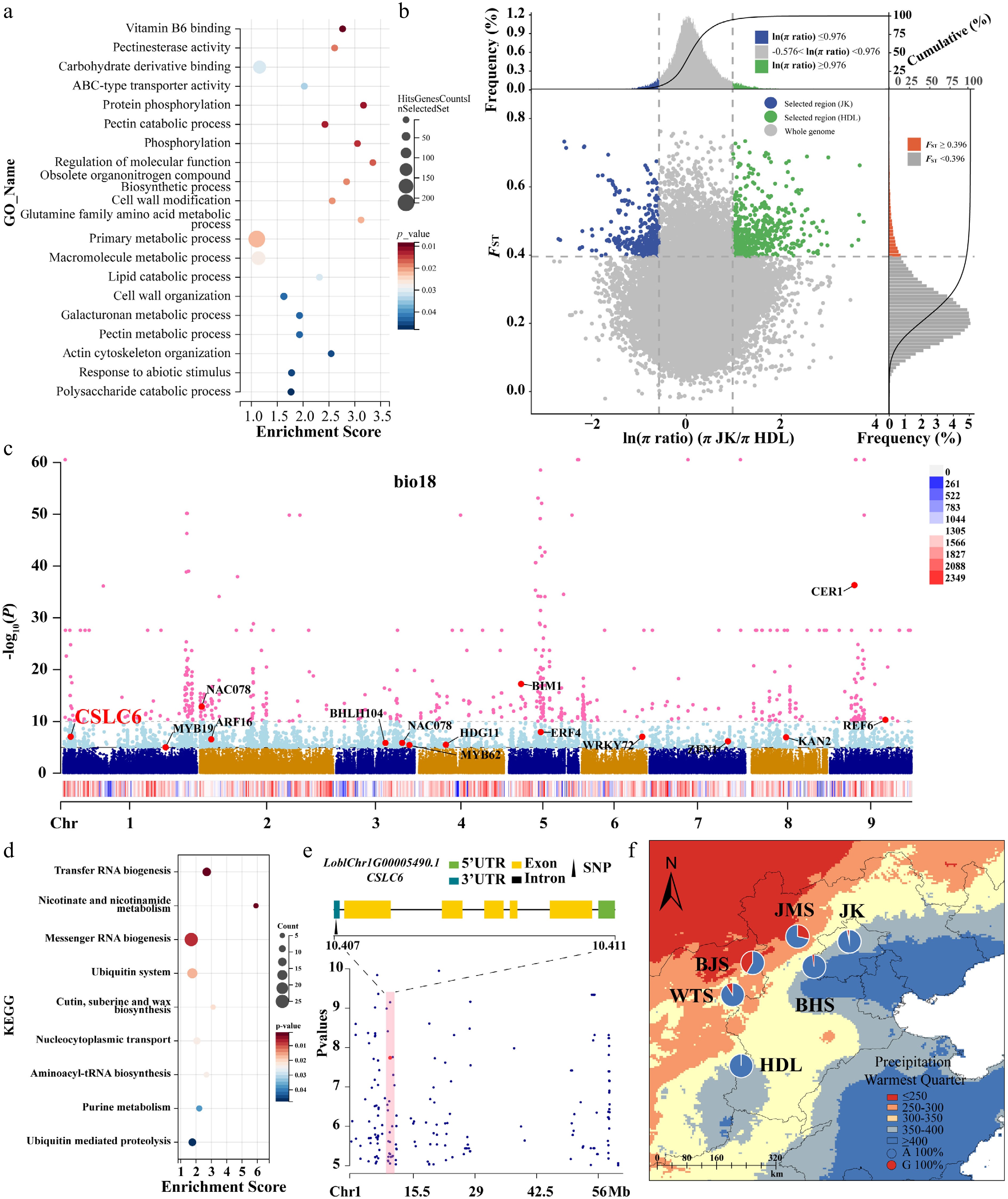
Figure 5. 

Selective sweeping analyses for the Northern JK and Southern HDL populations, along with genome-wide variation association analyses of Lonicera oblata. (a) GO enrichment results for genes containing selective candidate SNPs. The size and color of the circles represent the number of genes enriched in specific pathways and the degree of pathway enrichment, respectively. (b) Distribution of ln (π ratios) and F_ST values calculated in 100-kb windows with 10-kb steps. (c) The Manhattan plot of SNPs associated with the environmental variable bio18 across the entire genome estimated with LFMM. The vertical axis represents the p-value of the relationship between SNPs and bio18, ranging from 1 to 1.0e–60. The light blue and pink dots indicate the threshold p-value of 1.0e–5 and 1.0e–10, respectively. The colored strips with a red-blue gradient represent the density of SNPs on the chromosome. (d) KEGG enrichment results for genes containing selective candidate SNPs. (e) The location of the genes where the core SNPs are situated on Chr1. The black triangle indicates that the adaptive SNP is in the 3' UTR region of the gene. The red dots and shaded areas highlight the positions of the target SNPs within the locally magnified section of the Manhattan plot. (f) The genotype frequency distribution of core SNPs corresponding to precipitation gradients across different populations. Blue represents genotype A, while orange represents genotype G. The red and blue areas on the map indicate precipitation levels during the hottest season (bio18).

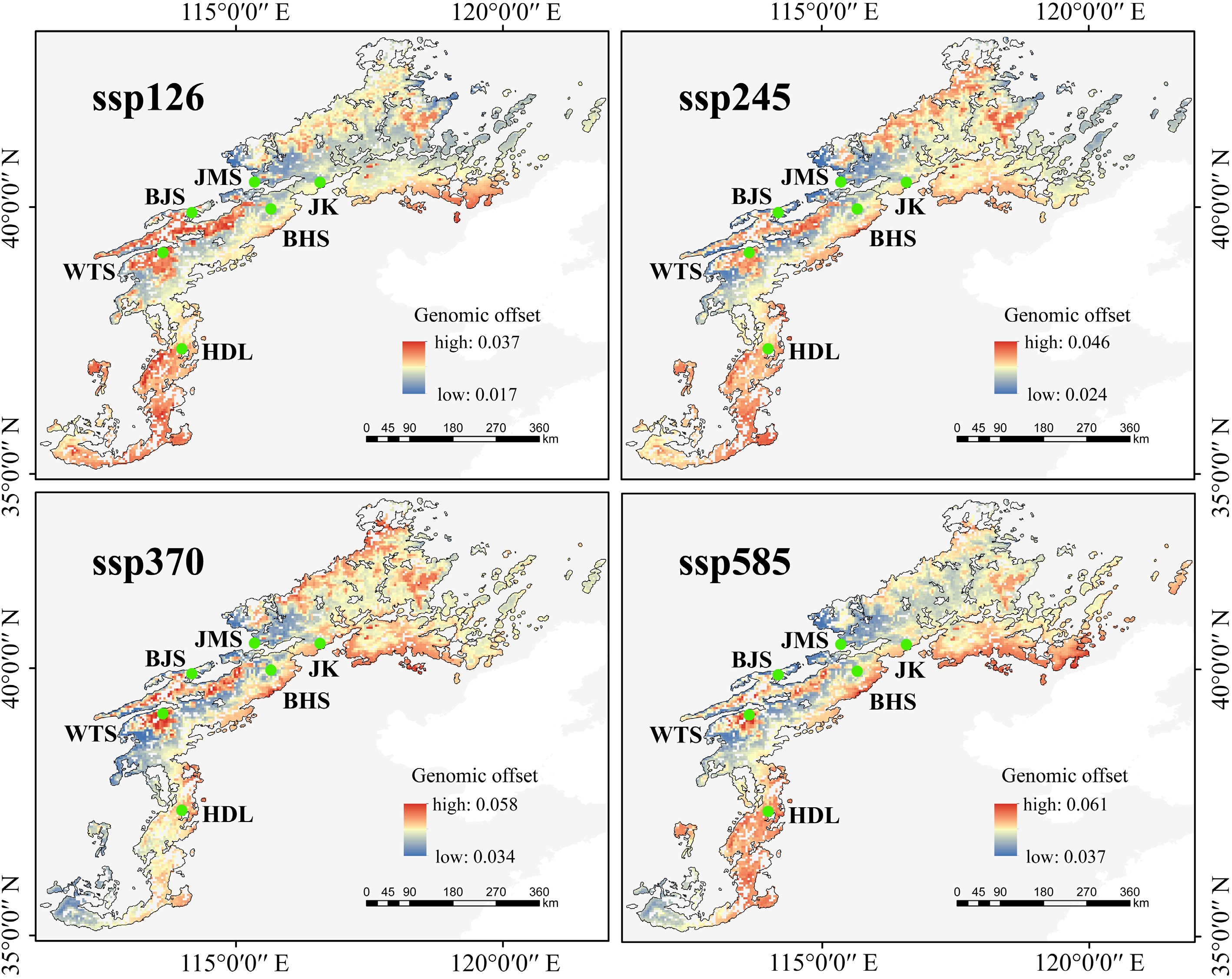
Figure 6. 

Predicted genomic offset of Lonicera oblata in response to future climate change (2081–2100) using the BCC-CSM2-MR model. Source: the National Platform for Common Geospatial Information Services (Tianditu), with review number GS(2024)0650. www.tianditu.gov.cn