-
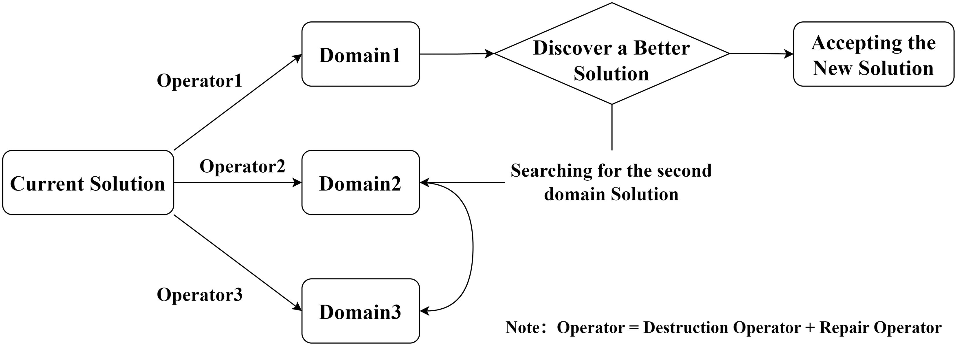
Figure 1.
Flowchart of the ALNS algorithm.
-
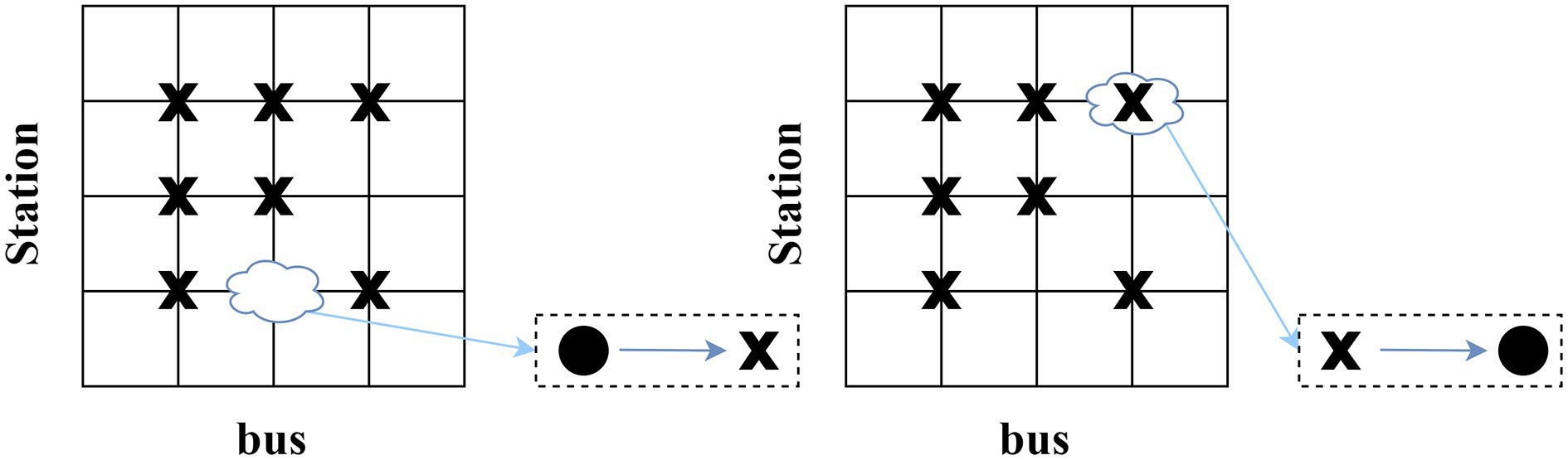
Figure 2.
Randomly skip/stop.
-
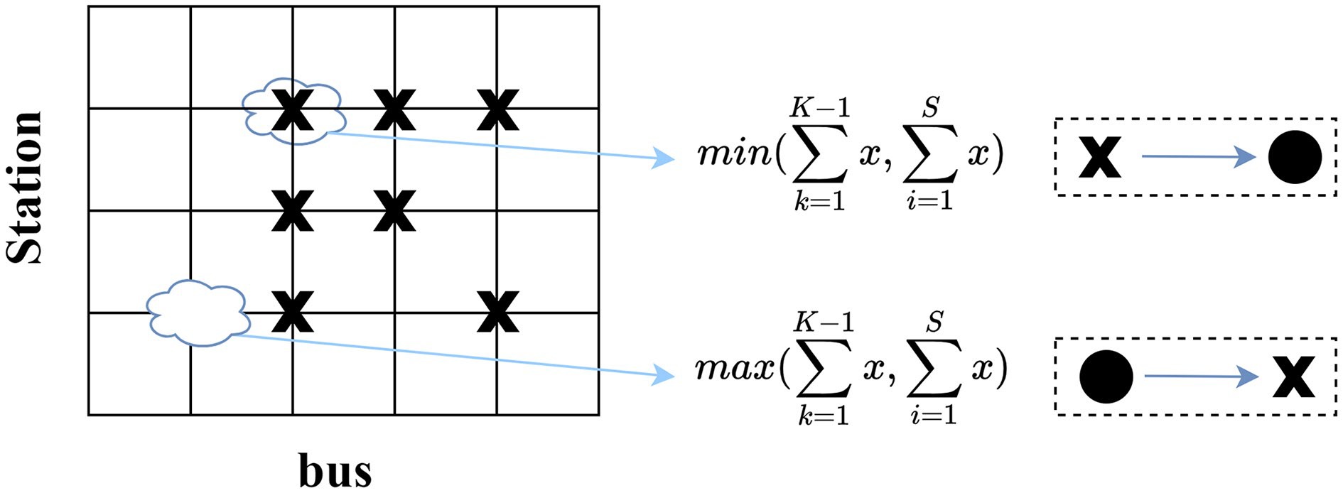
Figure 3.
Frequency_driven skip/stop.
-
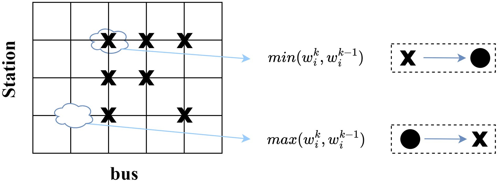
Figure 4.
Demand-driven skip/stop.
-
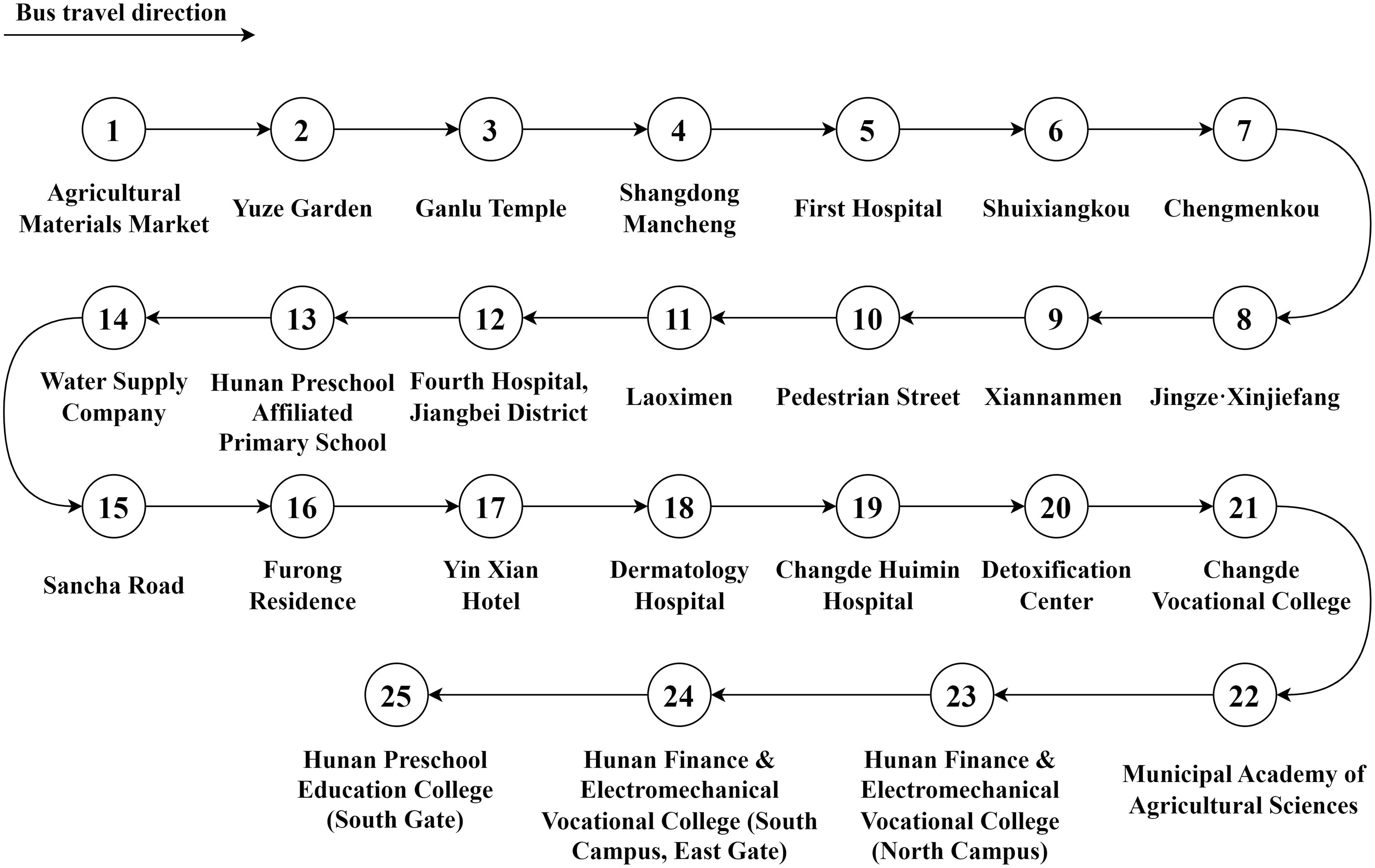
Figure 5.
Changde No.1 bus route map.
-
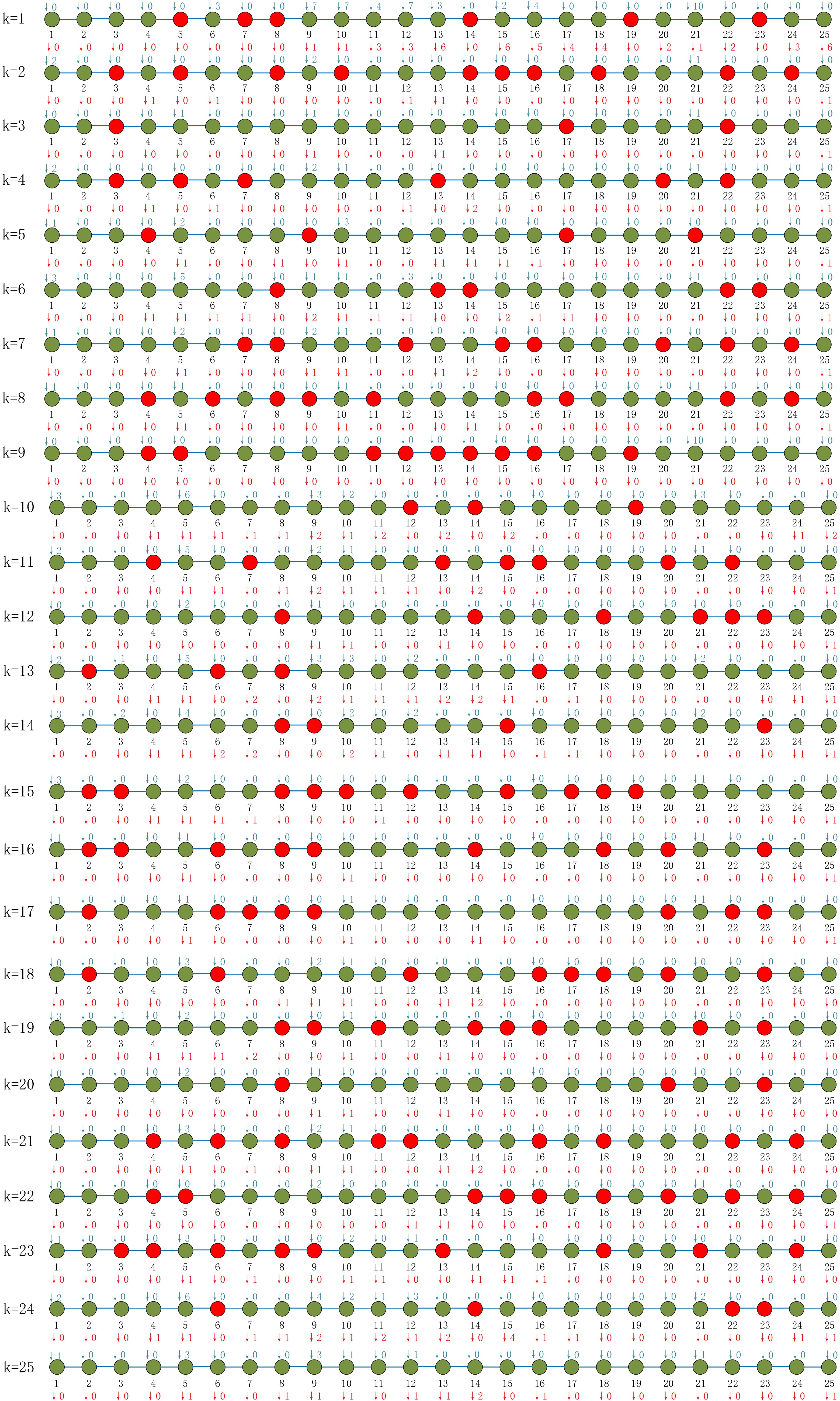
Figure 6.
Original scheduling skip station plan: Red stations indicate skipped stops, while green stations indicate stops. The upper number represents the number of boarding passengers, and the lower number represents the number of alighting passengers. In the first half of the route (stations 1–13), where passenger flow is relatively concentrated, buses stop more frequently.
-
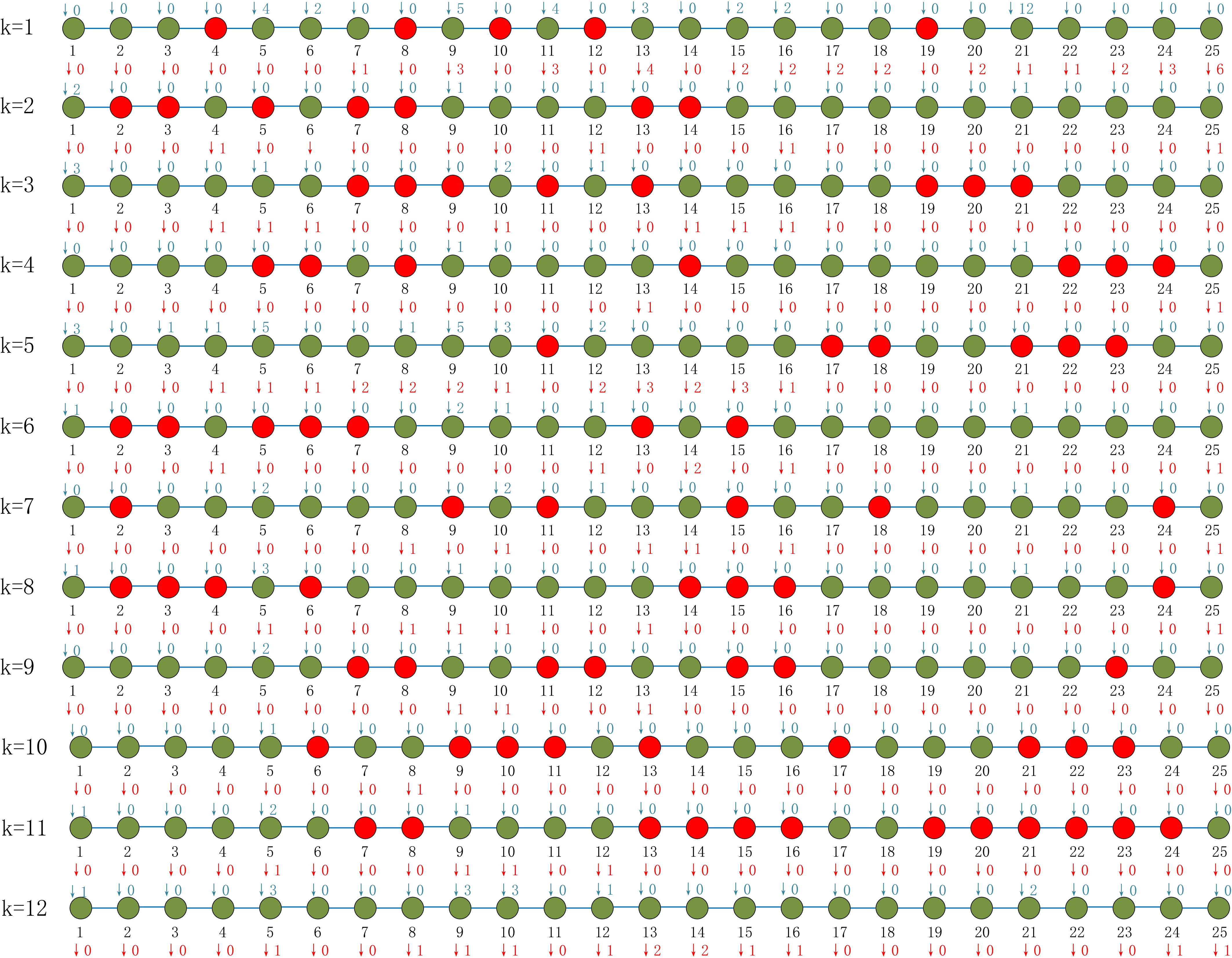
Figure 7.
Optimal skip-stop scheduling with reduced train frequency: Red and green markers indicate skipped and served stations, respectively, with each station labeled by the number of boarding and alighting passengers. The skip-stop pattern adapts to passenger flow: 'stop once, skip once' in high-flow upper sections and consecutive skipping in low-flow lower sections, with skipped stations evenly distributed along the route.
-
xxx Set S = {1, 2, ......, |S|}, represents a set of bus stops K = {1, 2, ......, |S|}, represents a set of vehicles within a service cycle Parameter ti The running time of public transportation from the i-th station to the i + 1st station P The duration of time that buses spend at each stop hmin The minimum safe time interval, known as the headway, that must be maintained between adjacent buses running on the same route hmax The maximum safe time interval, known as the headway, that must be maintained between adjacent buses running on the same route C The capacity of a bus, which typically refers to the maximum number of passengers it can safely transport β Input parameter to estimate the average waiting time for passengers at a bus stop who are anticipating the arrival of the next bus that can take them to their destination Decision variable $ x_{i}^{k} $ 0,1 variable, if K car stops at station i, take 1; otherwise, take 0 $ y_{ij}^{k} $ 0,1 variable, if the k-car stops at both i and j stations, take 1; otherwise, take 0 Intermediate variable $ {h}_{L} $ The regular interval of time between the arrivals of consecutive buses at a given stop or along a route $ A_{i}^{k} $ The precise moment when train K reaches station i, within a given operational schedule $ C_{i}^{k} $ The maximum number of passengers that can board the k train when it stops at station i Passenger related parameters and variable parameters $ {\lambda }_{ij} $ The number of passengers from station i to station j per unit time $ {u}_{i} $ Static risk rating of passengers boarding at station i Intermediate variable $ d_{ij}^{k} $ The number of passengers who want to board the K train from station i to station j when it stops $ r_{ij}^{k} $ The number of passengers who want to travel from station i to station j before the arrival of train K $ r_{i}^{k} $ The total number of waiting passengers at station i before the arrival of train K $ R_{ij}^{k} $ The number of passengers who may board the K train at station i and go to station j $ R_{i}^{k} $ The total number of people who may board the K train at station i $ b_{ij}^{k} $ The actual number of people boarding the K train at station i to go to station j $ b_{i}^{k} $ The total number of people actually boarding the K train at station i $ w_{ij}^{k} $ The number of passengers who are stranded at station i and want to go to station j after the departure of train k $ n_{i}^{k} $ The total number of passengers inside the train k after leaving the station i Decision variable $ D_{i}^{k} $ The total risk inside the vehicle at station i $ Q_{i}^{k} $ Risk of infection among passengers in the train upon arrival at station i Table 1.
Notations, input parameters, and variables.
-
No. Number of bus
runs/tripsRoute Average waiting time
for passengers (min)Solution method 1 |K| = 3 1 10 ALNS 2 |K| = 4 1 8 ALNS 3 |K| = 5 1 6 ALNS 4 |K| = 3 2 10 ALNS 5 |K| = 4 2 8 ALNS 6 |K| = 5 2 6 ALNS 7 |K| = 3 3 10 ALNS 8 |K| = 4 3 8 ALNS 9 |K| = 5 3 6 ALNS 10 |K| = 4 1 8 Gurobi 11 |K| = 4 2 8 Gurobi 12 |K| = 4 3 8 Gurobi Table 2.
Instances of numerical experiments.
-
Parameter Symbol Value Maximum capacity C 30 Travel time between stops (min) ti 2 Stopping time at stations (min) p Originating station: 5, Intermediate stations: 1, Terminating station: 0 Minimum headway time (min) hmin 4 Maximum headway time (min) hmax 12 Minimum service frequency per stop fmin 1 Time saving weight β1 0.4 Risk weight β2 0.6 Static risk value at stops μ 2 Number of iterations epochs 100 Weight updating step size pu 5 Annealing rate phi 0.9 Table 3.
Parameters settings in numerical experiments.
-
No. Time saved (min) Risk of transmission Objective function Maximum consecutive skipped stops (stations) Maximum no. of stranded passengers (persons) 1 −198 7,534 4,441.2 4 10 2 70 9,813 5,915.8 4 4 3 −163 15,813 9,422.6 5 19 4 45 5,557 3,352.2 4 11 5 −122 6,567 3,891.4 5 8 6 −106 6,910 4,103.6 5 10 7 −3,648 53,471 30,623.4 8 44 8 −1,648 73,253 43,292.6 7 34 9 −1,791 89,457 52,957.8 9 23 Table 4.
Results of the first set of numerical experiments.
-
No. Objective function Running time (s) 2 5,915.8 7.22 10 5,833.4 478.6 5 3,891.4 7.5 11 3,376.3 512.3 8 43,292.6 18.15 12 42,726.9 8,756 Table 5.
Results of the second set of numerical experiments.
-
Off \on 1 2 3 4 5 6 7 8 9 10 11 12 13 14 15 16 17 18 19 20 21 22 23 24 1 − − − − − − − − − − − − − − − − − − − − − − − − 2 4 − − − − − − − − − − − − − − − − − − − − − − − 3 10 0 − − − − − − − − − − − − − − − − − − − − − − 4 20 2 2 − − − − − − − − − − − − − − − − − − − − − 5 26 4 6 3 − − − − − − − − − − − − − − − − − − − − 6 20 5 11 6 6 − − − − − − − − − − − − − − − − − − − 7 10 4 14 12 15 2 − − − − − − − − − − − − − − − − − − 8 4 2 11 15 29 5 2 − − − − − − − − − − − − − − − − − 9 1 0 6 12 36 11 4 1 − − − − − − − − − − − − − − − − 10 0 0 2 6 29 14 7 3 4 − − − − − − − − − − − − − − − 11 0 0 0 3 15 11 9 5 8 3 − − − − − − − − − − − − − − 12 0 0 0 0 5 5 7 6 16 7 2 − − − − − − − − − − − − − 13 0 0 0 0 0 2 4 5 20 14 4 5 − − − − − − − − − − − − 14 0 0 0 0 0 0 2 3 16 17 8 11 1 − − − − − − − − − − − 15 0 0 0 0 0 0 0 0 8 14 11 22 1 1 − − − − − − − − − − 16 0 0 0 0 0 0 0 0 3 7 8 27 2 3 1 − − − − − − − − − 17 0 0 0 0 0 0 0 0 1 2 4 22 4 7 2 0 − − − − − − − − 18 0 0 0 0 0 0 0 0 0 0 2 11 2 9 4 2 0 − − − − − − − 19 0 0 0 0 0 0 0 0 0 0 0 4 1 7 5 3 0 0 − − − − − − 20 0 0 0 0 0 0 0 0 0 0 0 0 0 3 4 4 0 0 0 − − − − − 21 0 0 0 0 0 0 0 0 0 0 0 0 0 1 2 3 1 0 0 0 − − − − 22 0 0 0 0 0 0 0 0 0 0 0 0 0 0 0 2 0 2 1 1 1 − − − 23 0 0 0 0 0 0 0 0 0 0 0 0 0 0 0 0 0 0 1 1 3 0 − − 24 0 0 0 0 0 0 0 0 0 0 0 0 0 0 0 0 0 0 1 2 6 0 0 − 25 0 0 0 0 0 0 0 0 0 0 0 0 0 0 0 0 0 0 0 2 16 0 0 0 Table 6.
Passenger OD matrix during the research period.
-
Station number Static risk value Station number Static risk value 1 18 14 3 2 3 15 1 3 4 16 6 4 4 17 1 5 11 18 1 6 0 19 5 7 1 20 0 8 1 21 8 9 1 22 0 10 0 23 5 11 10 24 9 12 3 25 5 13 1 Table 7.
Static risk value of the site.
-
Parameter Symbol Value Number of buses/shift |K| 25 Number of stops |S| 25 Maximum capacity C 30 Travel time between stops (min) ti 2 Stopping time at stations (min) p Originating station: 5, Intermediate stations: 1, Terminating station: 0 Average waiting time of passengers per minute β 4.4 Minimum headway time (min) hmin 4 Maximum headway time (min) hmax 12 Minimum service frequency per stop fmin 1 Time saving weight β1 0.4 Risk weight β2 0.6 Number of iterations epochs 100 Weight updating step size pu 5 Annealing rate phi 0.9 Table 8.
Solving parameters.
-
Saved time Risk value Objective function 197 298,479 179,166.2 Table 9.
Original scheduling solution results.
-
Saved time Risk value Objective function 86 122,919 73,785.8 Table 10.
Scheduling solution results for reducing shifts.
-
$ {\beta }_{1} $ $ {\beta }_{2} $ Saved time Risk value Objective function 0/1 13 10,916 6,554.8 0.2/0.8 59 119,393 103,536.4 0.4/0.6 86 122,919 73,785.8 0.6/0.4 99 120,412 56,224.2 0.8/0.2 97 121,659 20,409.4 1/0 110 148,444 110 Table 11.
Weighing coefficient value.
Figures
(7)
Tables
(11)