-
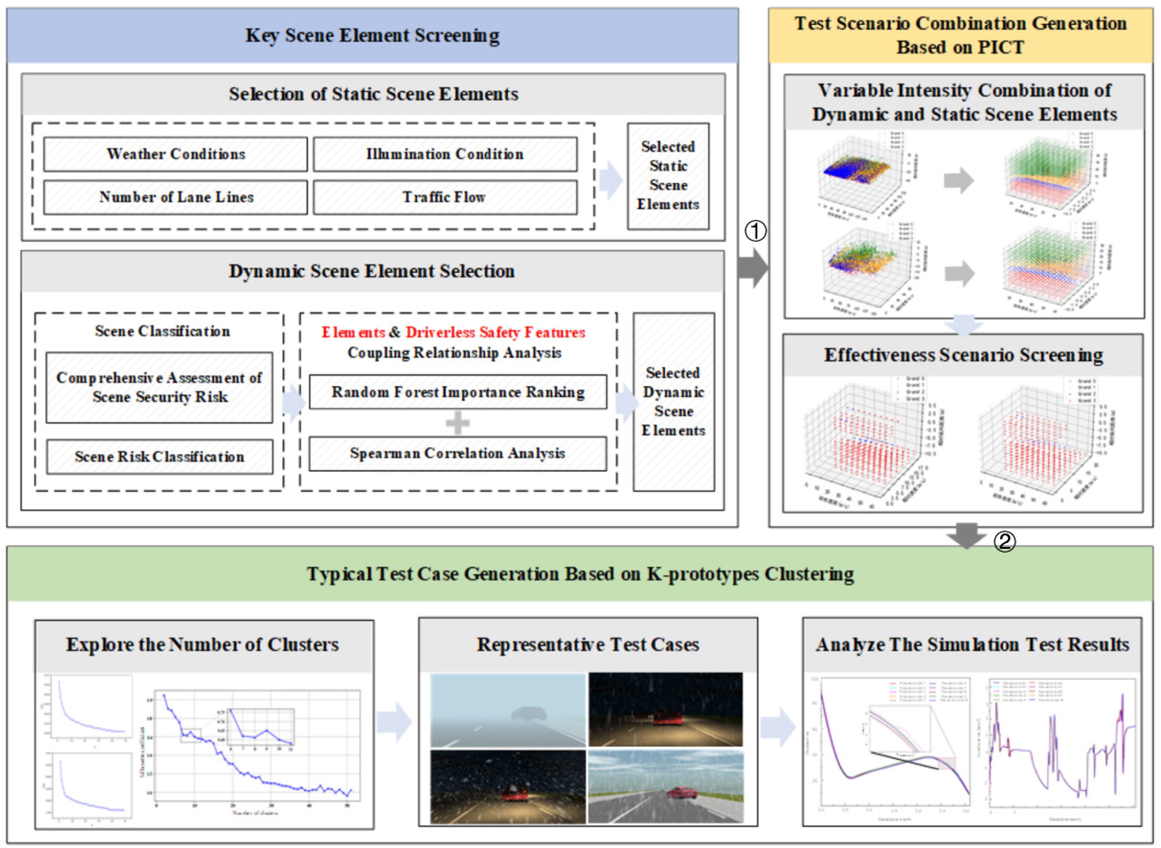
Figure 1.
Schematic of the test scenario construction process. ① selected dynamic and static scene parameters; ② filtered test scenarios.
-
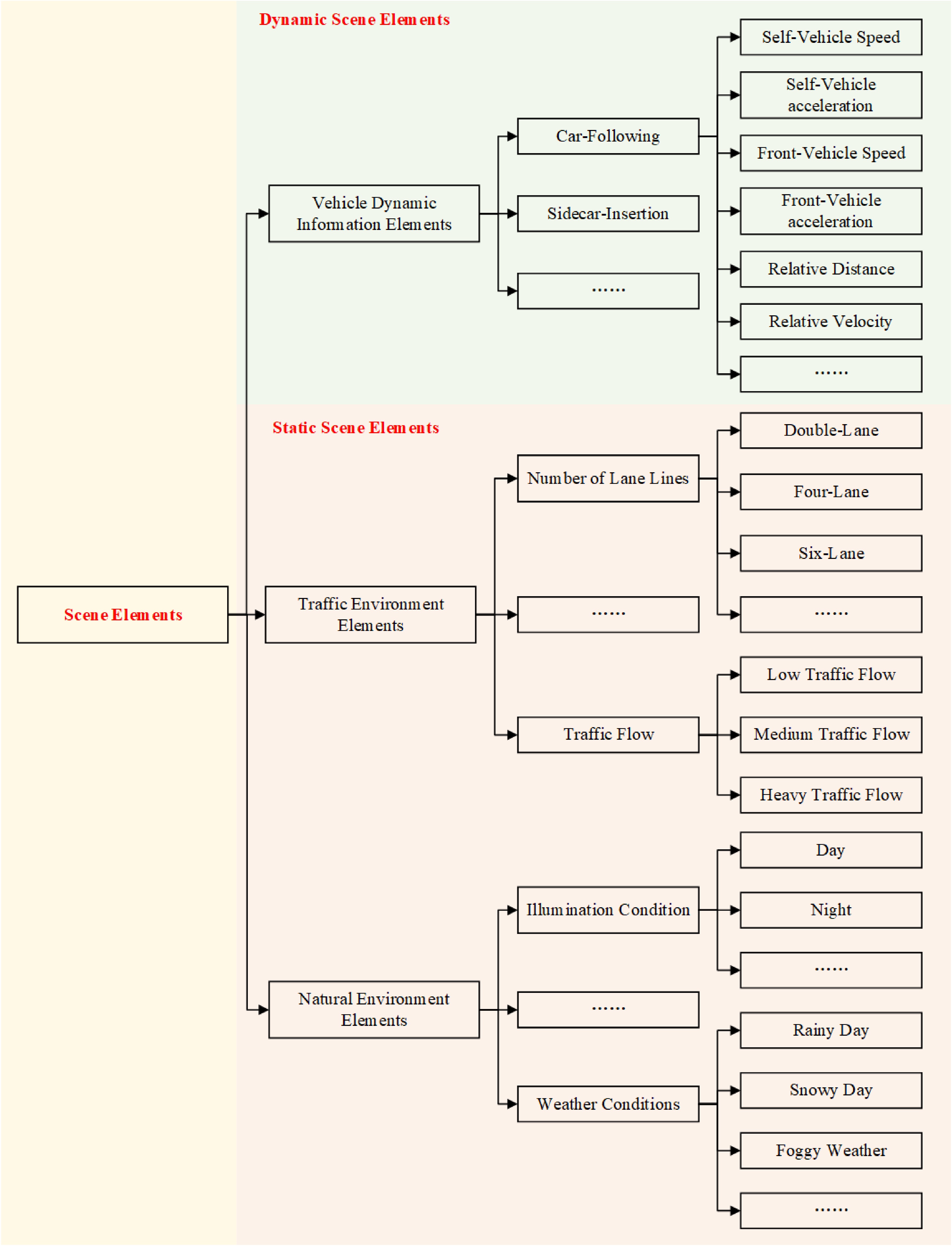
Figure 2.
Multidimensional decomposition of scenario elements.
-
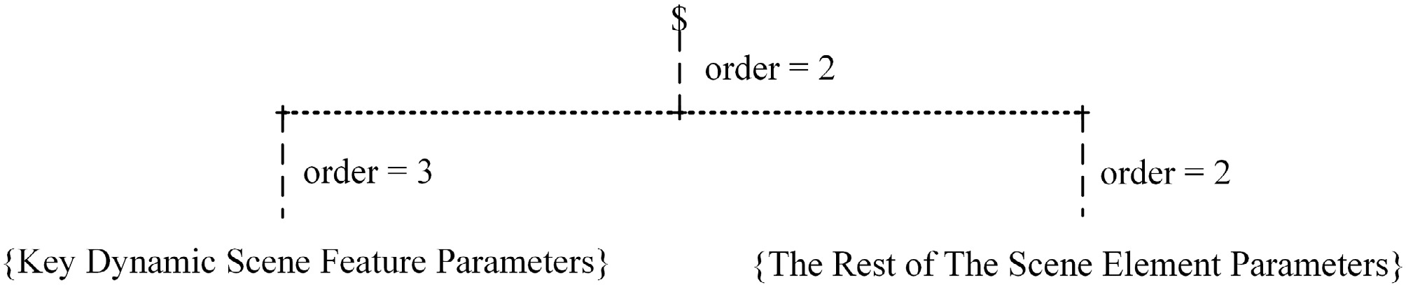
Figure 3.
Workflow of the variable-strength PICT combination testing method.
-
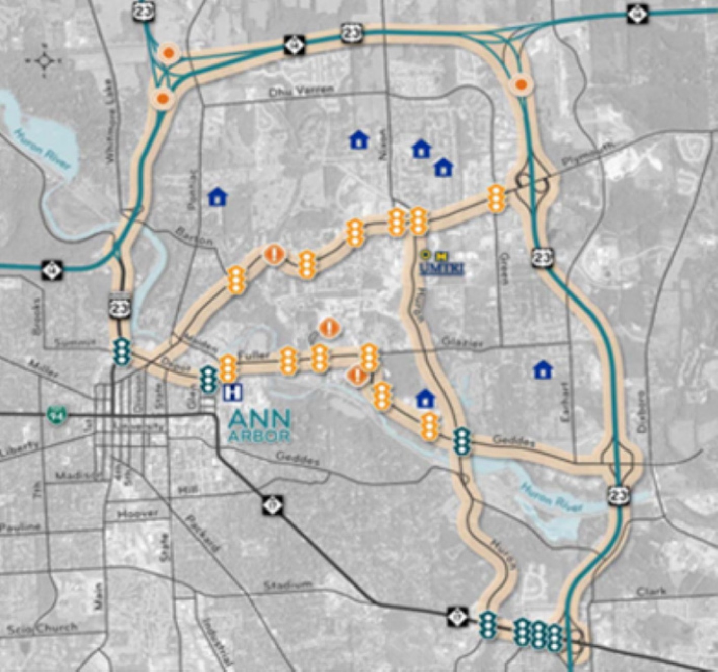
Figure 4.
Data collection area for the SPMD.
-
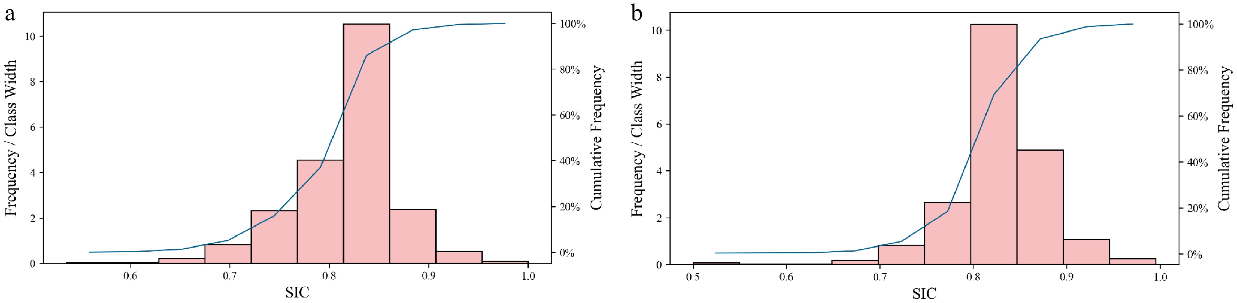
Figure 5.
PDF and CDF of SIC for extracted scenarios. (a) Car-following scenario. (b) Cut-in scenario.
-
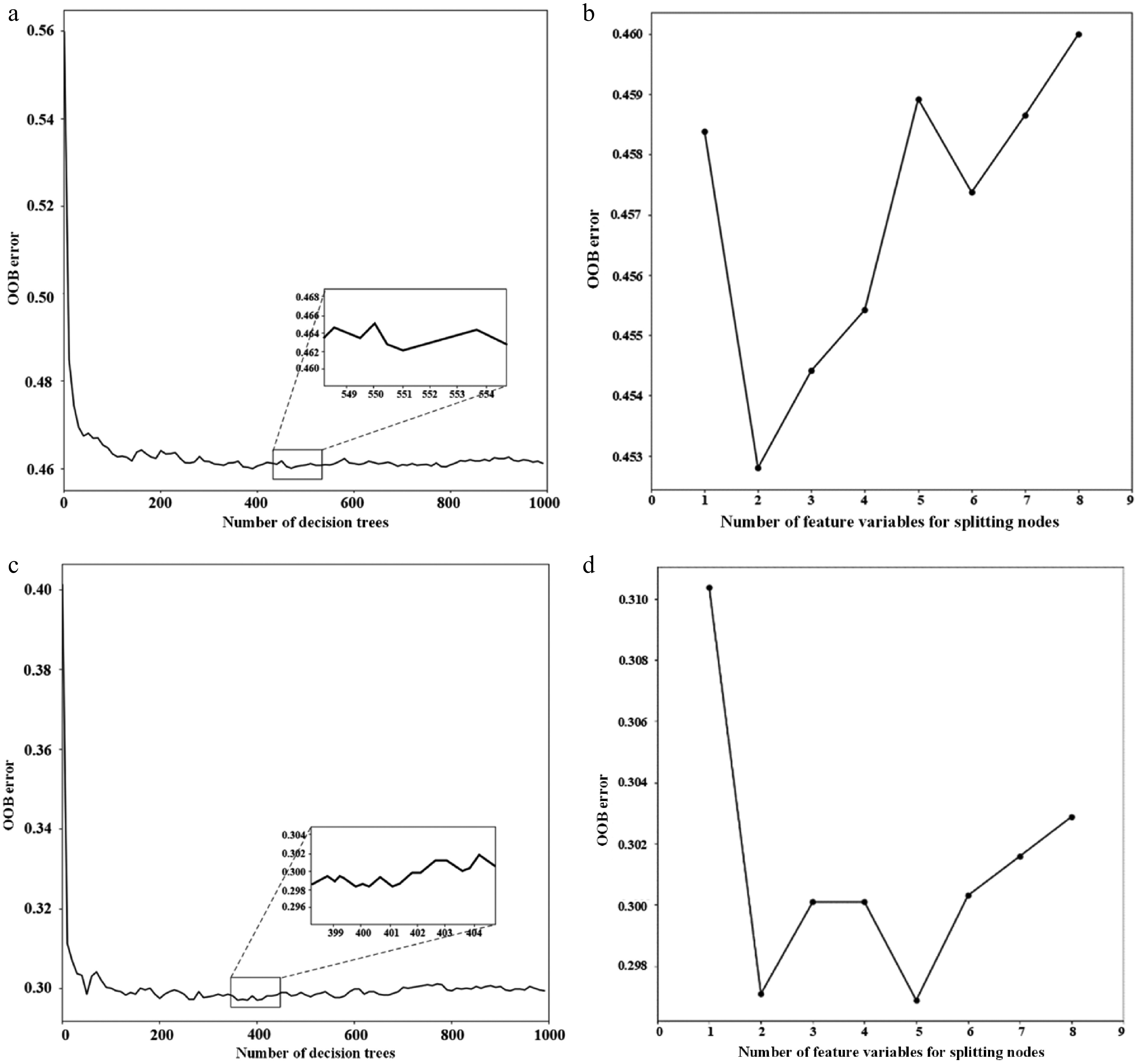
Figure 6.
Random forest parameter training process. (a) The number of decision trees for the car-following scenario. (b) The number of feature variables for the car-following scenario. (c) The number of decision trees for the cut-in car scenario. (d) The number of feature variables for the cut-in car scenario.
-
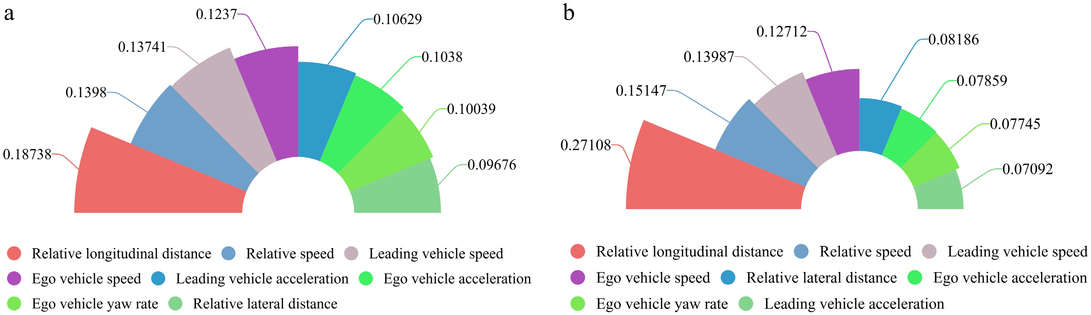
Figure 7.
Ranking of feature importance in RF. (a) Car-following scenario. (b) Cut-in scenario.
-
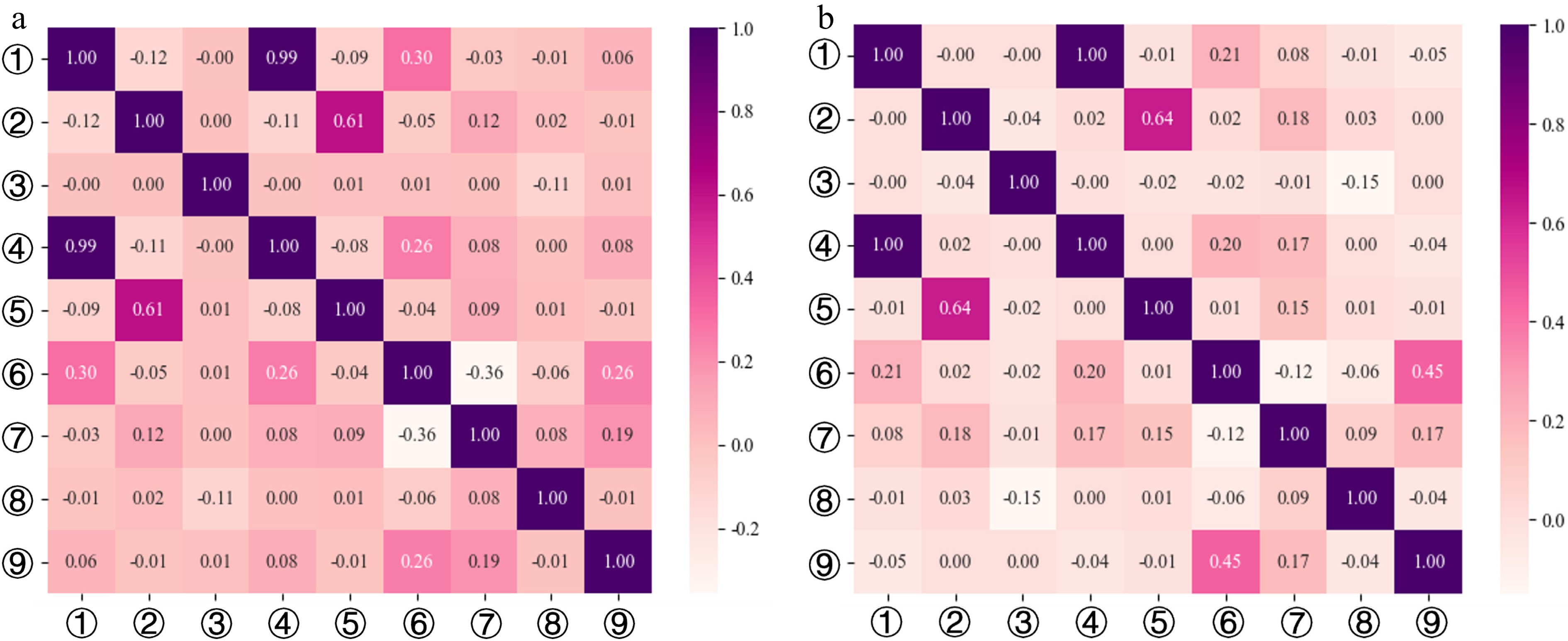
Figure 8.
Spearman correlation analysis results. (a) Car-following scenario. (b) Cut-in scenario. The meanings of the numbers in the figure are as follows: ① ego vehicle speed, ② ego vehicle acceleration, ③ ego vehicle yaw rate, ④ leading vehicle speed, ⑤ leading vehicle acceleration, ⑥ relative longitudinal distance, ⑦ relative speed, ⑧ relative lateral distance, and ⑨ SIC.
-
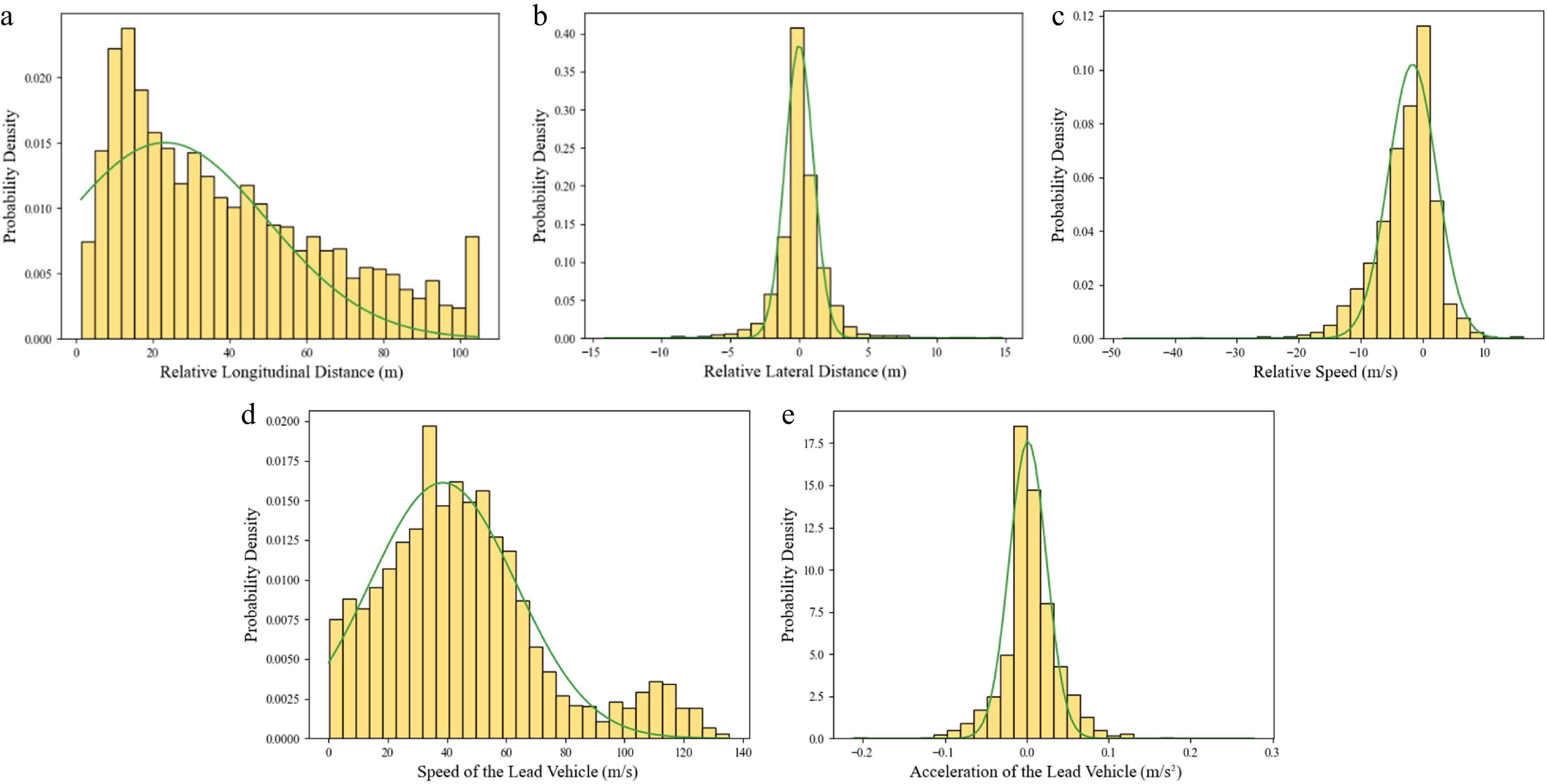
Figure 9.
Probability distribution of basic dynamic parameters for Grand 3 car-following scenario samples. (a) Relative longitudinal distance. (b) Relative lateral distance. (c) Relative speed. (d) Leading vehicle speed. (e) Leading vehicle acceleration.
-
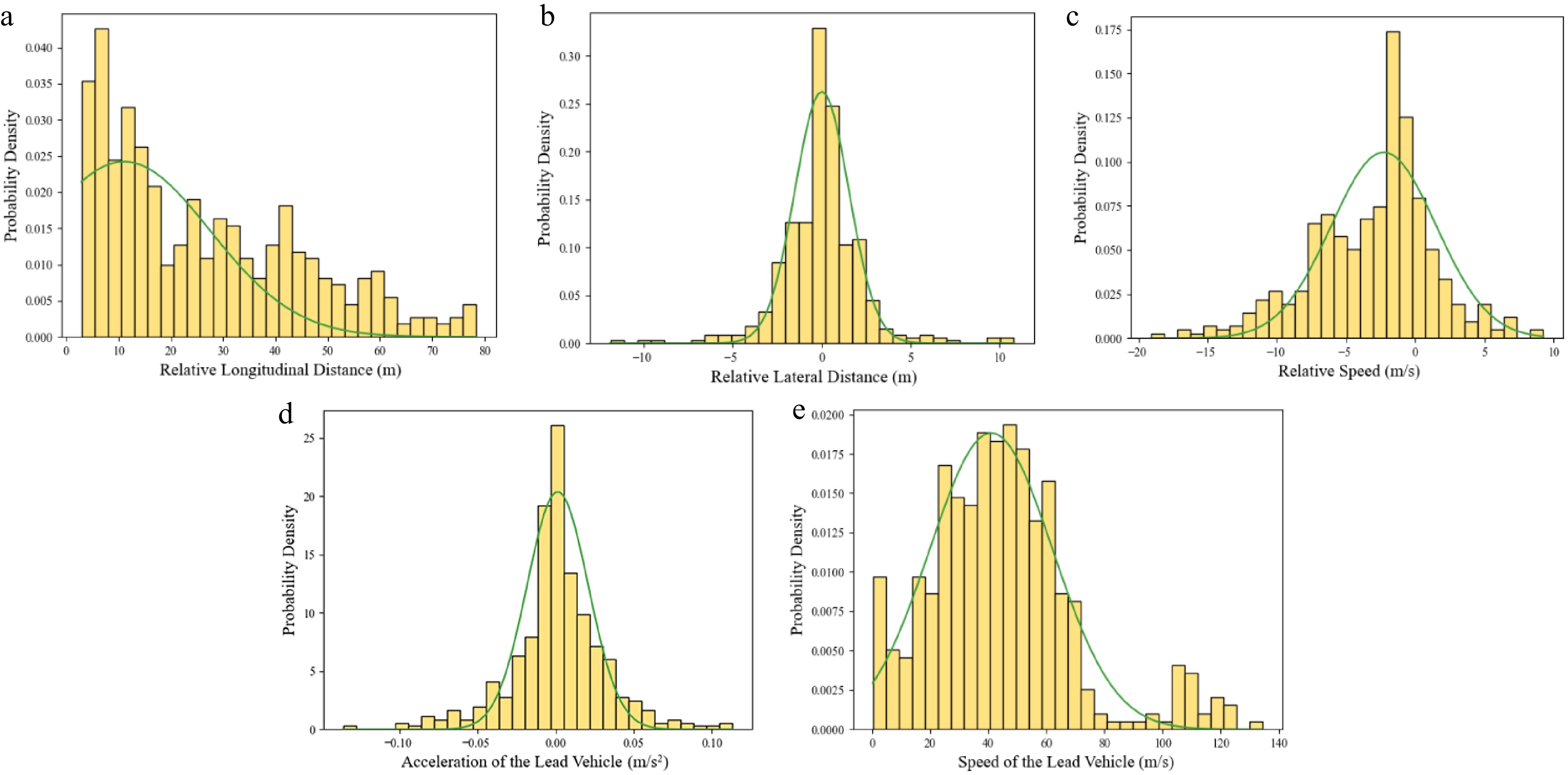
Figure 10.
Probability distribution of basic dynamic parameters for Grand 3 cut-in scenario samples. (a) Relative longitudinal distance. (b) Relative lateral distance. (c) Relative speed. (d) Leading vehicle speed. (e) Leading vehicle acceleration.
-
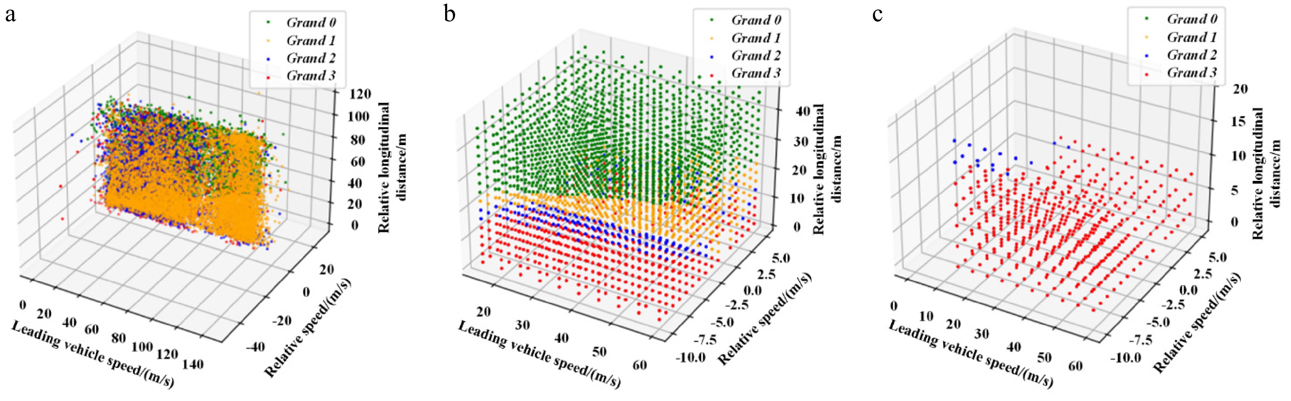
Figure 11.
Generation of car-following scenarios. (a) Original scenario. (b) PICT combined generated test scenario. (c) Filtered scenario.
-
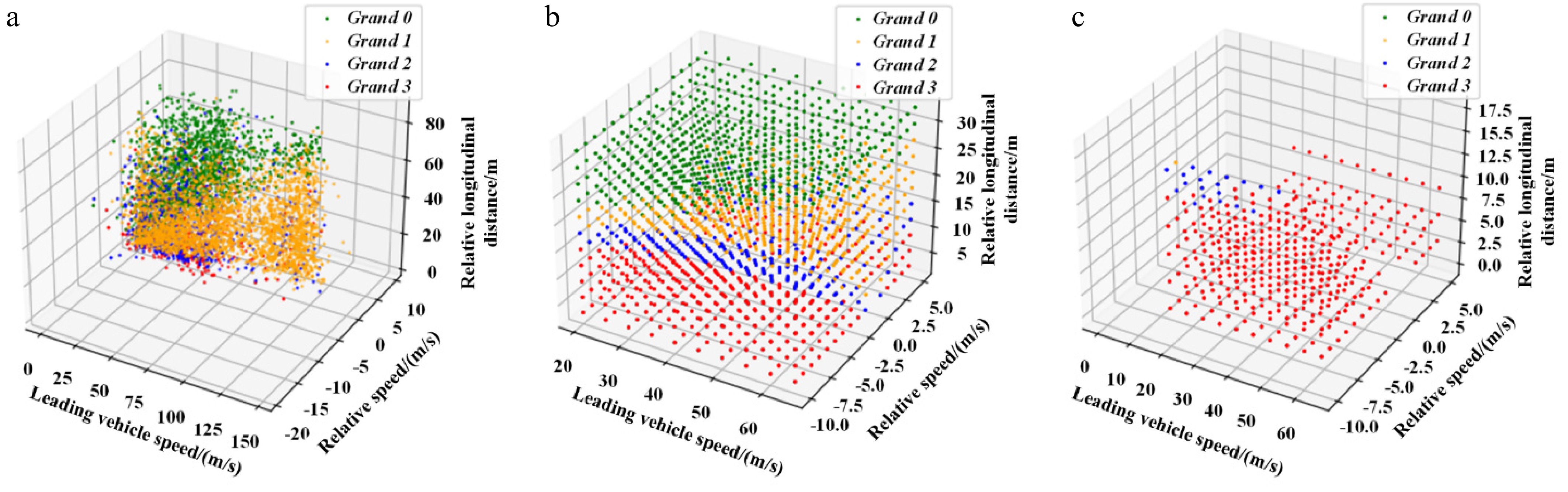
Figure 12.
Generation of cut-in scenarios. (a) Original scenario. (b) PICT combined generated test scenario. (c) Filtered scenario.
-
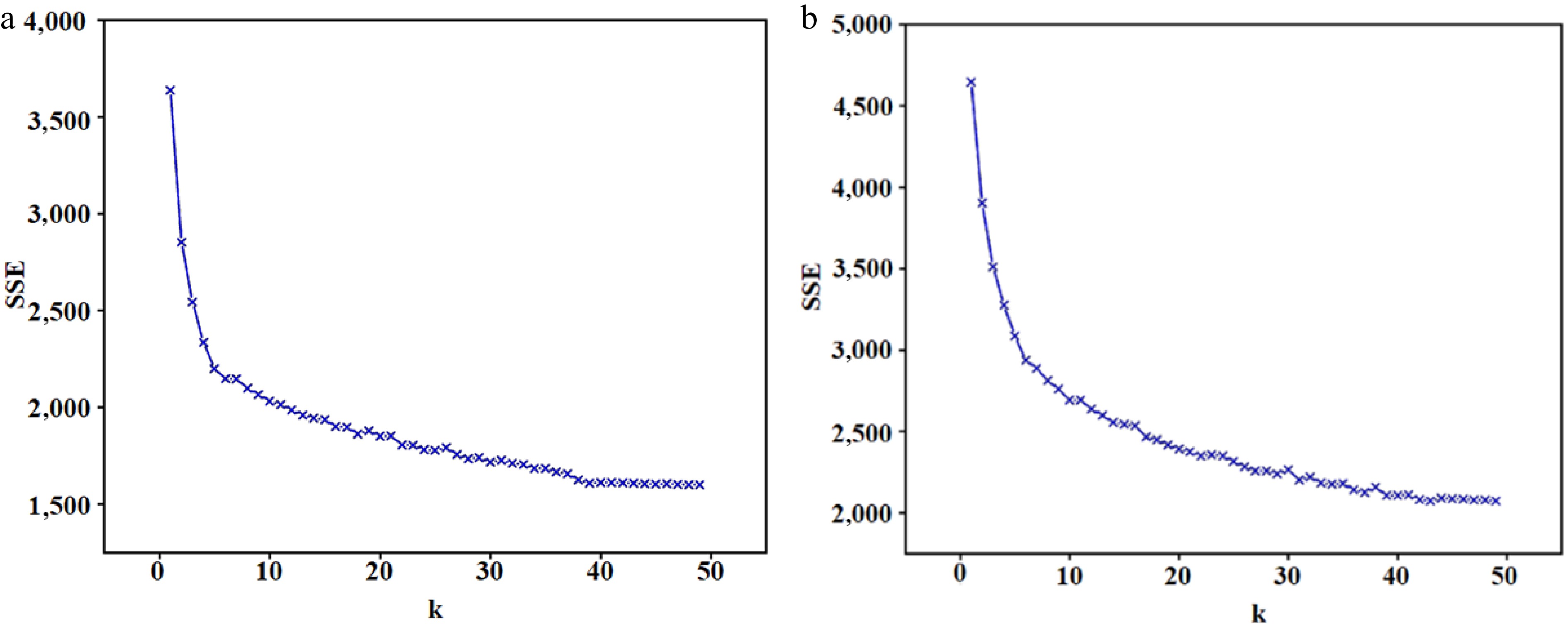
Figure 13.
Elbow plot of clustering. (a) Car-following scenario. (b) Cut-in scenario.
-
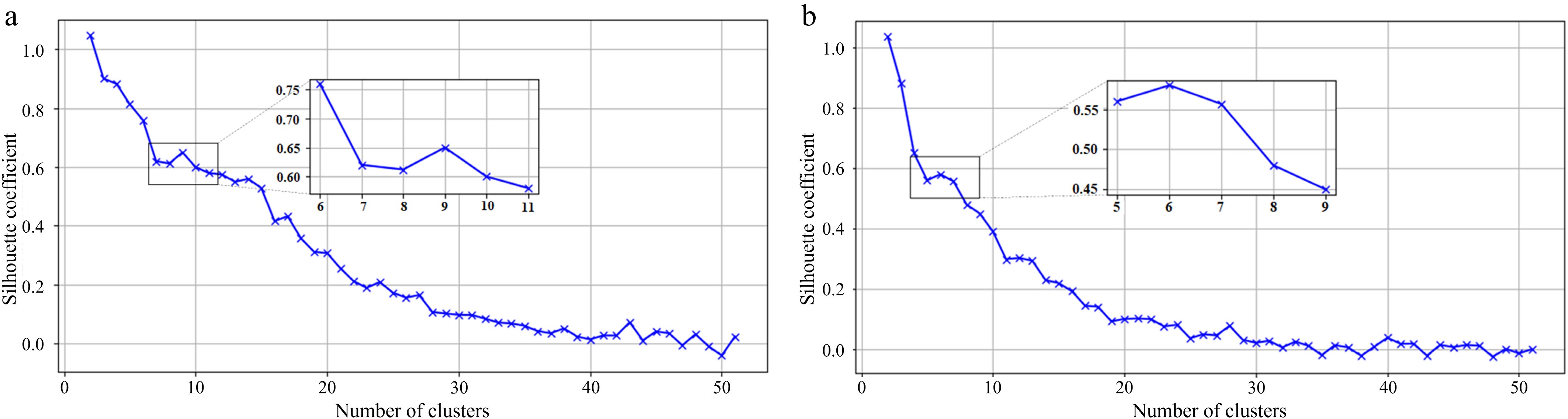
Figure 14.
Silhouette coefficient plot for clustering. (a) Car-following scenario. (b) Cut-in scenario.
-
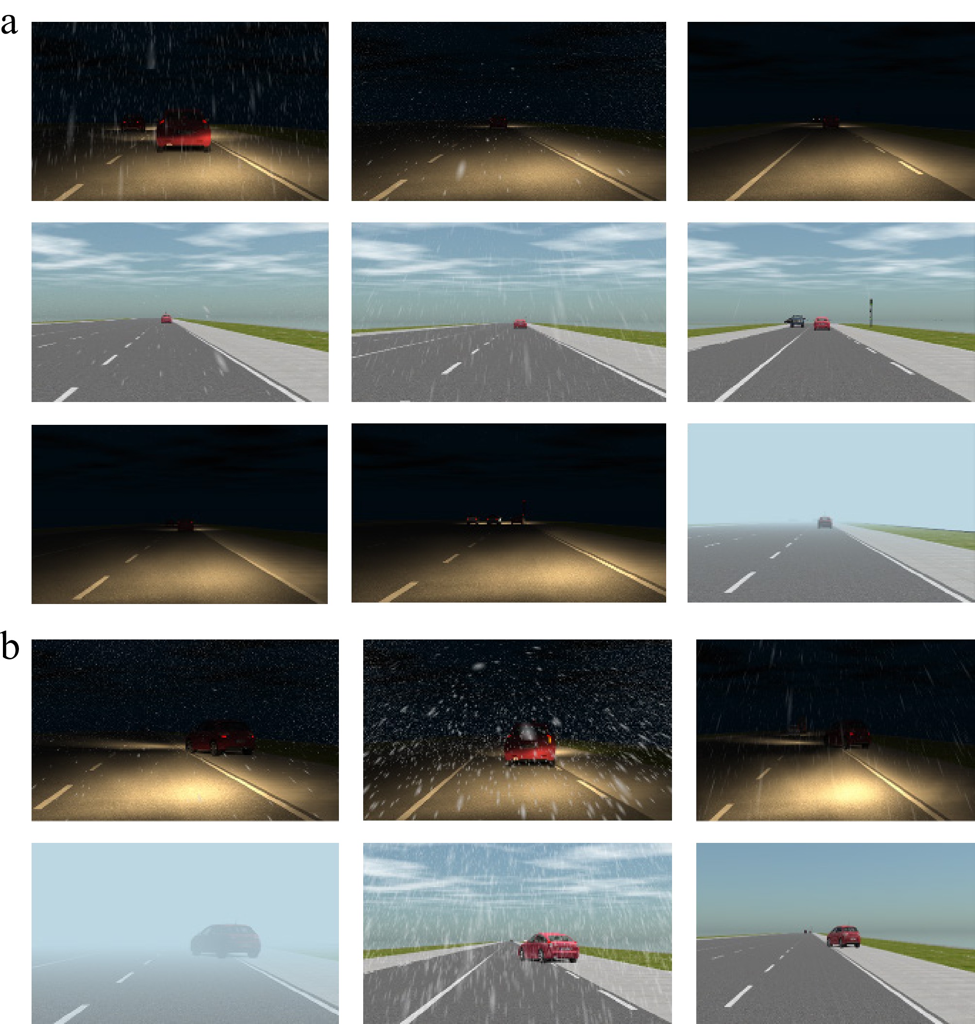
Figure 15.
Fifteen representative simulation test scenarios. (a) Car-following scenario. (b) Cut-in scenario.
-
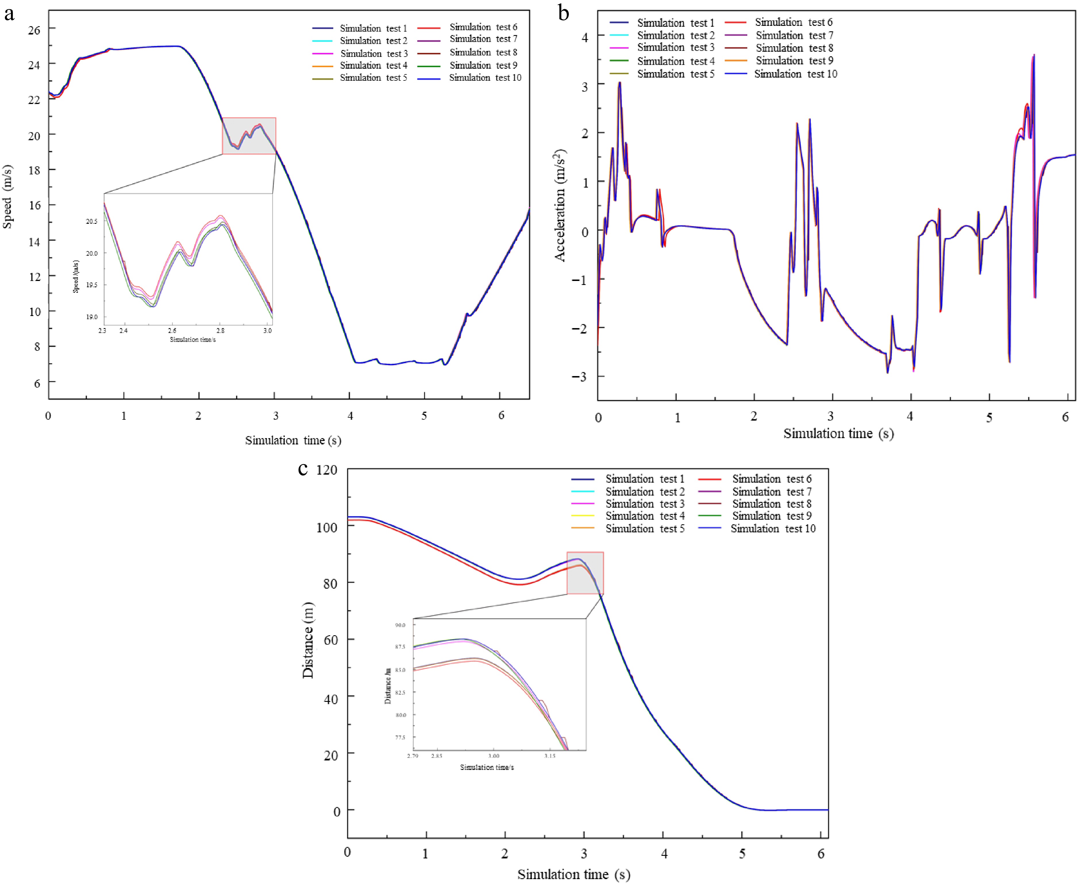
Figure 16.
Simulation test results for car-following Scenario 1. (a) Ego vehicle speed. (b) Ego vehicle acceleration. (c) Relative distance.
-
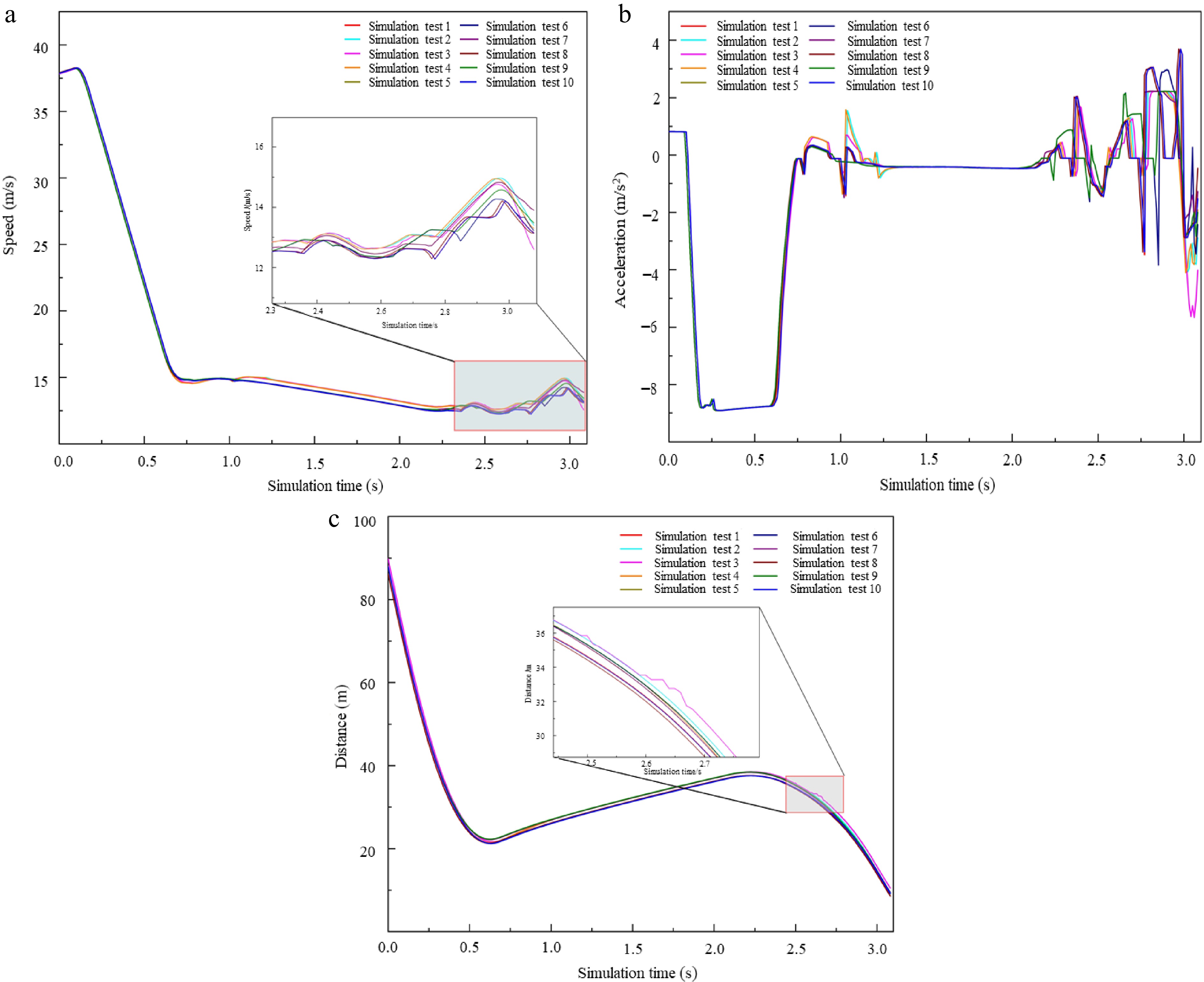
Figure 17.
Simulation test results for cut-in Scenario 1. (a) Ego vehicle speed. (b) Ego vehicle acceleration. (c) Relative distance.
-
Static scenario elements Parameter value Natural environment elements Weather
conditionsRainy Small, medium, large Snowy Small, medium, large Foggy Small, medium, large Clear day − Illumination condition Day, night Traffic environment elements Number of lane lines 2, 3, 4 Traffic flow Low, medium, high Table 1.
Parameter set for static scenario elements.
-
Screening index Screening condition TTC TTC < 2 s THW 20 m/s < Vx < 40 m/s THW < 0.01 × Vx + 0.1 Vx ≥ 40 m/s THW ≤ 0.5 s Table 2.
Scenario filtering criteria.
-
SIC range Safety impact level Number of scenarios SIC ≤ 0.7539 Grand 3 2,214 0.7539 < SIC ≤ 0.8025 Grand 2 3,233 0.8025 < SIC ≤ 0.8395 Grand 1 7,923 SIC > 0.8395 Grand 0 5,209 Table 3.
Car-following scenario risk level classification.
-
SIC range Safety impact level Number of scenarios SIC ≤ 0.7600 Grand 3 428 0.7600 < SIC ≤ 0.8004 Grand 2 724 0.8004 < SIC ≤ 0.8488 Grand 1 2,986 SIC > 0.8488 Grand 0 1,680 Table 4.
Cut-in scenario risk level classification.
-
Fitting parameter Mean ( $ \mu $ Standard deviation ( $ \sigma $ Relative longitudinal distance 23.48 26.58 Relative lateral distance 0.03 1.03 Relative speed −2.74 5.03 Leading vehicle speed 38.59 24.75 Leading vehicle acceleration 0.0011 0.0225 Table 5.
Normal distribution fit of key parameters for car-following scenarios.
-
Fitting parameter Mean ( $ \mu $ Standard deviation ( $ \sigma $ Relative longitudinal distance 11.03 16.47 Relative lateral distance 1.52 0.02 Relative speed −2.27 3.79 Leading vehicle speed 40.98 21.18 Leading vehicle acceleration 0.0012 0.0196 Table 6.
Normal distribution fit of key parameters for cut-in scenarios.
-
Scenario elements Parameter value Car-following Cut-in Relative longitudinal distance (1.5, 46.5) 1.5 m discrete (3, 33) 3 m discrete Relative lateral distance 0 (1, 3) 0.5 m/s discrete Relative speed (−10, 5) 1 m/s discrete (−10, 5) 1 m/s discrete Leading vehicle speed (15, 60) 5 m/s discrete (15, 60) 5 m/s discrete Leading vehicle acceleration 0 0 Table 7.
Vehicle dynamic information elements set.
-
Scenario
typeScenario WC IC NL TF LD
(m)LAD
(m)RS
(m/s)LS
(m/s)LA
(m/s2)Car-following 1 CD N 6 H 19.5 0 0 30 0 2 R-M D 4 L 4.5 0 3 15 0 3 CD N 4 M 34.5 0 0 25 0 4 S-S D 6 M 10.5 0 −6 50 0 5 CD N 2 L 7.5 0 −9 35 0 6 R-S D 2 H 13.5 0 −10 55 0 7 S-M N 6 L 22.5 0 0 55 0 8 R-M N 4 H 4.5 0 −4 40 0 9 F-S D 6 H 1.5 0 −8 30 0 Cut-in 1 S-L N 2 L 18 1.5 0 22 0 2 CD D 6 M 6 2.5 0 60 0 3 R-M N 4 M 15 1 −10 60 0 4 S-S N 6 H 24 2.5 −8 17 0 5 R-L D 2 H 12 3 −10 40 0 6 F-L D 4 L 33 2 0 20 0 WC, weather conditions; IC, illumination condition; NL, number of lane lines; TF, traffic flow; LD, relative longitudinal distance; LAD, relative lateral distance; RS, relative speed; LS, leading vehicle speed; LA, leading vehicle acceleration. In WC, CD represents clear day. If shown in the form 'a-b', a represents weather (R, S, F, for rainy, snowy, foggy, respectively), and b represents severity (S, M, L, for small, medium, large, respectively). In IC, D and N represent day and night, respectively. In TF, L, M, and H represent low, medium, and high, respectively. Table 8.
Fifteen types of typical test scenarios.
Figures
(17)
Tables
(8)