-
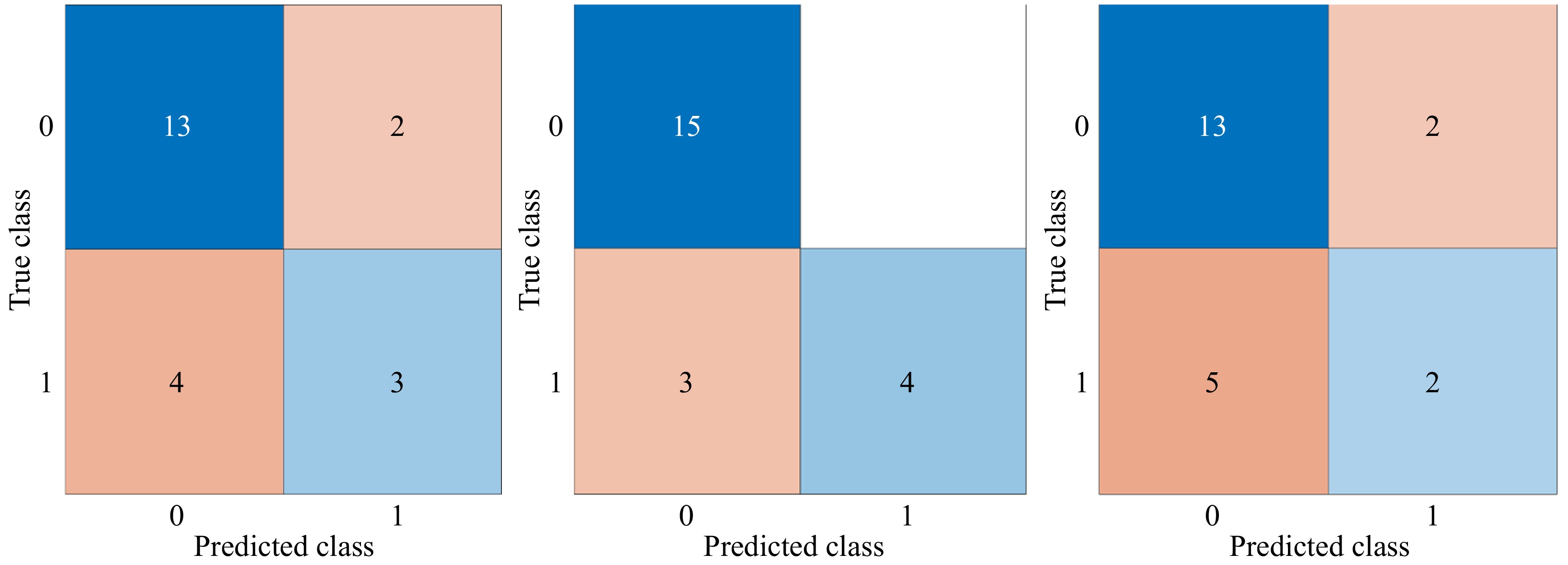
Figure 1.
Test results of confusion matrix for SVM, ET, NN.
-
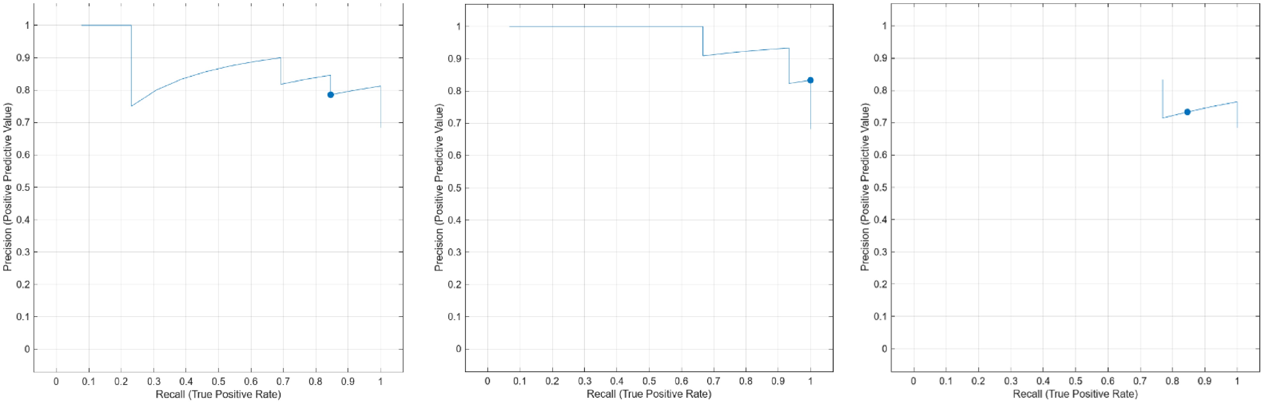
Figure 2.
Test Precision-Recall Curve for SVM, ET, NN.
-
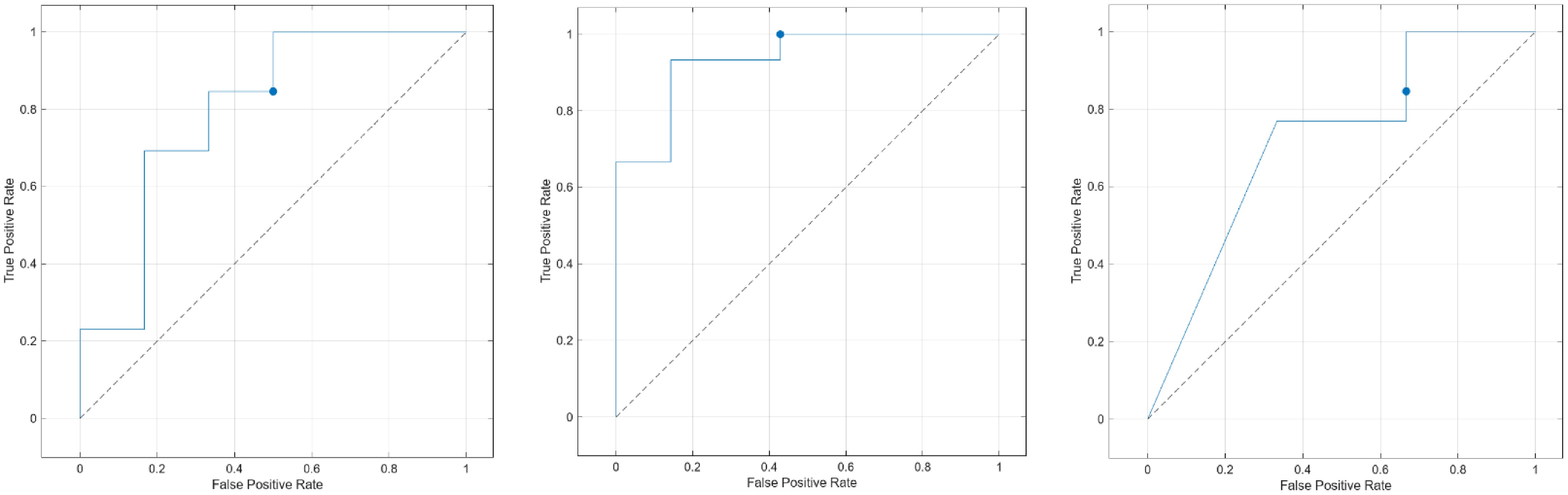
Figure 3.
Test ROC curve for SVM, ET, and NN.
-
Ref. Method Data Performance metrics Variables used Results [2] Stacking combined model, GBDT, Random Forest (RF), SVM, LSTM, CNN 549 accident reports (Fujian Sea area) Accuracy (0.912), precision (0.910), recall (0.912), F1 (0.904) Characteristic variables (x) Stacking model provided superior accuracy over traditional ML. [6] Data-driven BN, Fisher optimization, PMM, KNN, CatBoost 10-year maritime data (2014–2024) Accuracy (95.37%), CatBoost/RF/KNN > 85% Ship type, gross tonnage, length, power, wind, weather, speed BN model demonstrates high accuracy in severity predictions under imperfect data. [28] RF, XGBoost, LightGBM, NN, SVM, SMOTE 617 incidents (fishing vessels) RF AUC (0.93), Accuracy (0.8455) Tonnage, speed ratio, Delta-V, collision angle, relative speed SMOTE effectively balanced data; RF model was superior to other tested models. [3] Data-driven BN (TAN) 402 global accident records (2017–2021) Accuracy (92.86% for
2-year model), recall,
F-measure24 RIFs (ship type, age, location, weather, etc.) Data-driven TAN model uncovers more intricate relationships than expert-driven models. [22] AutoML (29 algorithms), LightGBM, XGBoost, RF 9,025 Norwegian accidents (1981–2020) Best accuracy (0.647), AUC (0.81) Vessel type, length, tonnage, navigation waters Light Gradient Boosted Trees Classifier was the best performing model. [12] LR, DT, RF, ET, NN, LightGBM, XGBoost, CatBoost, SMOTE, XAI 1,294 reports from seven global agencies Accuracy (0.7954 for LightGBM/ET), AUC (0.8469) Human factors, vessel characteristics, environment, management Feature selection and data balancing significantly enhance prediction accuracy. [21] BN (K2 and EM algorithms), ANN 2,080 tanker accident reports (USCG) Accuracy (75.96%), AUC (0.722) Accident type, vessel age, size, waterway type Vessel age and size are critical factors in predicting oil spill occurrence. [29] Decision Tree (CART), Tree Augmented Naive Bayes (TAN) 1,468 oil spill instances (USCG) Accuracy (0.669), AUC (0.704) Vessel type, accident type, waterway, severity TAN outperforms standard Naive Bayes; vessel type is a major spill predictor. [10] AutoML, LightGBM, RF, XGBoost 9,226 accidents + 57 weather variables Accuracy (0.7143 combined), AUC (Log Loss 0.816) Wind speed, visibility, temperature, moon phase Integrating high-resolution weather data improves accident risk prediction by ~6%. [5] RF, NB, SVM, XGBoost,
Adaboost, LightGBM,
FS (PGI-SDMI)MARIFD (1,294 reports) Accuracy (0.8555), AUC (0.9226) 68 RIFs (human, ship, env, management) The two-stage feature selection method achieves highest stability and precision. [15] ARIMAX, ARIMA Historical time series of accidents RMSE, MAE, MAPE, R2 Collision, machinery damage, weather conditions ARIMAX (multivariate) provides more accurate trends than simple ARIMA. [30] GBDT, LightGBM, XGBoost, ARFuse (ARM) Marine accidents risk influential factors database UAR (unweighted average recall) Management, regulation, human error, ship type ARFuse method optimizes the identification of hidden feature contributions to severity. [31] Systematic Literature Review (Survey) Review of 100+ publications Identification of research gaps (black box models) Vessel management, MetOcean, incident history Shift from naval mechanical analysis to human-environmental multi-factorial risk. [7] Ordered Logistic Regression 1,128 accident reports Significance (p < 0.05) Ship type, size, age, location, weather Ship age and crew experience are statistically significant severity predictors. [20] Data-driven TAN-BN 1,294 reports (AIF database) Mutual information values 35 third-level AIFs (human, ship, env) Human violation and ship age are top-ranked determinants of severity. [17] Augmented BN, Naive BN 350 waterborne records MDL score, ROC curve 20 risk variables (tonnage, speed, visibility) Augmented BN provides better structural fit and predictive power than standard Naive BN. [32] Grey-Markov prediction model Historical frequency data Prediction accuracy rates Minor, general, and major accidents Combinatorial models outperform single models in frequency forecasting. [33] SVM (Linear/Gaussian), Naive Bayes, Text Mining MAIB investigation reports (text) F-measure (SVM-Gaussian: 74%) Connective words, causal transitions NLP algorithms can effectively extract causal relations from textual reports. [34] kNN, XGBoost, Random Search optimization NISA/Korea Coast Guard data Precision, recall, F1 score Time, location, voyage data kNN-based data retrieval outperforms k-d tree and Ball tree methods. [35] Dynamic BN 460 emergency text cases Marginal probabilities X1–X13 (operational, environmental) Dynamic BN captures temporal risk evolution across different time slices. [19] CART, RF, Bayesian Optimization (BO) Text-mined accident reports Precision (0.8564), specificity, F1-score Ship type, age, accident type BO-RF model achieves highest precision for consequence scenario prediction. [8] ANOVA, Clustering, NN 300–617 Spanish SAR incidents Error histogram, predictor importance Ship type, crew, length, year Crew number and vessel length are the primary determinants of accident type. [23] LR, DT, RF, NN, GBT, Stochastic GBT 13,000 traffic records (New Orleans) Accuracy (SGBT: 0.983), sensitivity Traffic, environment, waterway SGBT models provide a highly reliable warning mechanism for maritime authorities. [36] GBDT, XGBoost, LightGBM, KMeans-SMOTE Marine accidents reports UAR (unweighted average recall) Tonnage, speed, weather features KMeans-SMOTE combined with GBDT shows optimal UAR scores for imbalanced data. Table 1.
Review of maritime accident studies.
-
Variable name Description Data type Unique value count Min. Max. Range Mean Median Mode Standard deviation Variance Date of occurrence The date when the accident happened Numerical 6 2015 2020 5 2016.96 2017 2015 1.52 2.31 Occurrence severity The severity of the accident Categorical 2 0 1 1 0.33 0 0 0.47 0.22 Occurrence with ship(s) The name(s) or description
of the vessel(s) involved in
the accident.Categorical 8 1 8 7 3.75 4 1 2.29 5.26 Ship/craft type The type of vessel Categorical 8 1 8 7 4.22 4 2 2.20 4.84 Lives lost - Total The total number of fatalities in the accident. Numerical 9 0 19 19 0.35 0 0 1.55 2.39 People injured - Total The total number of injured people. Numerical 10 0 37 37 0.59 0 0 2.85 8.14 Pollution Environmental pollution caused by the accident Categorical 2 0 1 1 0.12 0 0 0.32 0.10 Age on casualty The age of the vessel at the time of the accident Numerical 56 0 65 65 18.50 16 18 13.55 183.59 Length overall The total length of the vessel Categorical 205 5 179.985 179.980 11,889.11 176 225 29,806.39 888,420,805.75 Flag state The country where the ship is registered. Categorical 47 1 47 46 25.88 30 30 12.91 166.65 Sea area of occurrence The maritime zone where the accident took place Categorical 10 1 10 9 3.88 4 1 2.57 6.59 Wind force Wind intensity during the accident Categorical 13 0 12 12 4.20 4 5 2.35 5.51 Sea state Wave height and sea conditions Categorical 10 0 9 9 3.06 3 4 1.83 3.34 Natural light Lighting conditions at the time of the accident Categorical 3 1 3 2 1.69 2 2 0.63 0.40 Visibility Visibility range Categorical 5 1 5 4 2.36 2 2 0.66 0.44 Weather conditions General weather Categorical 5 1 5 4 2.55 2 2 0.75 0.56 Bad weather Whether adverse weather contributed to the accident Categorical 3 0 2 2 0.69 1 0 0.71 0.50 Education Crew's education/training level Categorical 2 0 1 1 0.41 0 0 0.49 0.24 Inappropriate behavior Human error led to the accident Categorical 2 0 1 1 0.45 0 0 0.50 0.25 Equipment Equipment failure or inadequacy contributed
to the accident.Categorical 2 0 1 1 0.48 0 0 0.50 0.25 Table 2.
Study dataset and descriptive analysis results.
-
Date of
occurrenceOccurrence
severityOccurrence
with ship(s)Ship/craft
typeLives lost -
TotalPeople injured -
totalPollution Age on
casualtyLength
overallFlag
stateSea area of
occurrenceWind
forceSea
stateNatural
lightVisibility Weather
conditionsBad
weatherEducation Inappropriate
behaviorEquipment Date of occurrence 1.00 −0.03 −0.13 −0.03 −0.07 0.03 −0.14 0.07 0.09 0.02 0.17 0.08 0.09 0.01 0.12 0.11 0.14 −0.06 −0.11 −0.02 Occurrence severity −0.03 1.00 0.15 0.18 0.32 −0.01 0.13 0.15 −0.07 0.02 0.09 0.07 0.07 −0.06 0.15 0.03 0.07 −0.04 −0.07 −0.08 Occurrence with ship(s) −0.13 0.15 1.00 0.00 0.19 0.05 0.02 −0.07 −0.06 0.07 −0.04 −0.10 −0.04 −0.05 −0.09 −0.08 −0.16 −0.01 −0.25 0.12 Ship/craft type −0.03 0.18 0.00 1.00 −0.10 0.14 0.14 0.33 0.06 −0.10 0.04 −0.01 −0.05 0.06 0.03 0.23 0.06 −0.01 0.10 0.01 Lives lost - Total −0.07 0.32 0.19 −0.10 1.00 0.00 −0.05 −0.02 −0.02 −0.12 −0.06 0.03 0.08 −0.10 0.23 −0.01 0.10 0.05 −0.07 −0.04 People injured - Total 0.03 −0.01 0.05 0.14 0.00 1.00 −0.06 0.02 −0.02 0.04 −0.04 −0.15 −0.11 0.10 −0.17 0.14 0.08 0.07 0.01 −0.02 Pollution −0.14 0.13 0.02 0.14 −0.05 −0.06 1.00 −0.02 −0.03 −0.02 −0.04 0.05 0.07 −0.02 −0.03 0.00 0.08 −0.07 0.06 −0.01 Age On Casualty 0.07 0.15 −0.07 0.33 −0.02 0.02 −0.02 1.00 −0.05 −0.03 0.03 0.16 0.00 0.09 0.00 0.11 0.13 0.04 0.00 −0.03 Length overall 0.09 −0.07 −0.06 0.06 −0.02 −0.02 −0.03 −0.05 1.00 −0.04 0.05 −0.07 −0.05 −0.05 0.00 −0.02 −0.04 −0.01 0.10 −0.09 Flag State 0.02 0.02 0.07 −0.10 −0.12 0.04 −0.02 −0.03 −0.04 1.00 −0.03 −0.10 −0.05 −0.03 −0.14 0.00 −0.01 −0.08 −0.02 −0.11 Sea area of occurrence 0.17 0.09 −0.04 0.04 −0.06 −0.04 −0.04 0.03 0.05 −0.03 1.00 0.04 0.16 −0.10 −0.04 0.09 0.11 −0.02 0.09 −0.05 Wind force 0.08 0.07 −0.10 −0.01 0.03 −0.15 0.05 0.16 −0.07 −0.10 0.04 1.00 0.69 −0.03 0.20 0.00 0.59 −0.09 −0.08 0.09 Sea state 0.09 0.07 −0.04 −0.05 0.08 −0.11 0.07 0.00 −0.05 −0.05 0.16 0.69 1.00 −0.05 0.14 0.02 0.59 −0.09 −0.12 0.03 Natural light 0.01 −0.06 −0.05 0.06 −0.10 0.10 −0.02 0.09 −0.05 −0.03 −0.10 −0.03 −0.05 1.00 0.06 −0.08 −0.02 0.11 −0.12 0.00 Visibility 0.12 0.15 −0.09 0.03 0.23 −0.17 −0.03 0.00 0.00 −0.14 −0.04 0.20 0.14 0.06 1.00 0.03 0.05 −0.12 −0.19 0.03 Weather conditions 0.11 0.03 −0.08 0.23 −0.01 0.14 0.00 0.11 −0.02 0.00 0.09 0.00 0.02 −0.08 0.03 1.00 0.51 −0.02 0.05 −0.13 Bad weather 0.14 0.07 −0.16 0.06 0.10 0.08 0.08 0.13 −0.04 −0.01 0.11 0.59 0.59 −0.02 0.05 0.51 1.00 −0.07 −0.08 0.03 Education −0.06 −0.04 −0.01 −0.01 0.05 0.07 −0.07 0.04 −0.01 −0.08 −0.02 −0.09 −0.09 0.11 −0.12 −0.02 −0.07 1.00 0.27 −0.08 Inappropriate behavior −0.11 −0.07 −0.25 0.10 −0.07 0.01 0.06 0.00 0.10 −0.02 0.09 −0.08 −0.12 −0.12 −0.19 0.05 −0.08 0.27 1.00 −0.16 Equipment −0.02 −0.08 0.12 0.01 −0.04 −0.02 −0.01 −0.03 −0.09 −0.11 −0.05 0.09 0.03 0.00 0.03 −0.13 0.03 −0.08 −0.16 1.00 Table 3.
Pearson correlation matrix of dataset variables.
-
Algorithm Formula/key concept Explanation ET $ \begin{gathered}\hat{y}=majority\_ vote({h}_{1}\left(x\right),\\{h}_{2}\left(x\right),\ldots ..,{h}_{n}\left(x\right))\end{gathered} $ h1 (x): each represents a decision tree trained on different data subsets or features. Predictions are combined through majority voting. SVM $ f\left(x\right)=sign\left({w}^{T}x+b\right) $ w: Weight vector, x: Input feature vector, b: Bias term. SVM finds the optimal hyperplane that maximizes the margin between classes. Kernels can be used to transform non-linear data into a linear separable form. NN $ y=f\left(Wx+b\right) $
(for a single-layer example)W: Weight matrix, x: Input vector, b: Bias term, f: Activation function (e.g., ReLU, sigmoid). NN consists of layers of interconnected nodes and can model complex relationships. Deep learning models use multiple hidden layers. Table 4.
Classification algorithms and explanations.
-
Metric Formula Explanation Accuracy $ \dfrac{TP+TN}{TP+TN+FP+FN} $ Proportion of total predictions that were correct. Total cost $({\mathrm{FP}} \times {\mathrm{C}}_{{\mathrm{FP}}}) + ({\mathrm{FN}} \times {\mathrm{C}}_{{\mathrm{FN}}}) $ Total cost of false positives and false negatives based on their respective costs. Error rate $ \dfrac{FP+FN}{TP+TN+FP+FN}=1-Accuracy $ Proportion of total predictions that were incorrect. Precision $ \dfrac{TP}{TP+FP} $ Proportion of positive predictions that were actually correct. Recall $ \dfrac{TP}{TP+FN} $ Proportion of actual positives that were correctly identified by the model. F1 score $ 2\times \dfrac{Precision\times Recall}{Precision+Recall} $ Harmonic mean of precision and recall; balances both metrics. TP (true positive): correctly predicted positive instances; TN (true negative): correctly predicted negative instances; FP (false positive): incorrectly predicted positive instances; FN (false negative):iIncorrectly predicted negative instances; C_FP, C_FN: cost assigned to false positive and false negative predictions, respectively. Table 5.
Performance metrics and explanations.
-
Observations Percentage Training data 201 90% Test data 22 10% Total 223 100% Table 6.
The count and percentage of observations for training and test datasets.
-
No. Features MRMR No. Features Kruskal-Wallis No. Features ANOVA No. Features Chi2 1 FlagState 0.1695 1 LivesLostTotal 37.2502 1 LivesLostTotal 12.4176 1 LivesLostTotal 35.2632 2 LivesLostTotal 0.1254 2 Pollution 4.3902 2 Pollution 4.4197 2 ShipCraftType 8.7494 3 Pollution 0.0125 3 OccurrenceWithShips 4.0363 3 OccurrenceWithShips 3.9258 3 OccurrenceWithShips 8.0179 4 OccurrenceWithShips 0.0100 4 Visibility 3.3583 4 Visibility 3.6051 4 Pollution 4.4079 5 AgeOnCasuality 0.0099 5 ShipCraftType 3.1645 5 ShipCraftType 3.1648 5 WeatherConditions 3.6584 6 WeatherConditions 0.0084 6 SeaState 2.9925 6 AgeOnCasullaty 2.9968 6 SeaAreaOfOccurrence 3.5726 7 ShipCraftType 0.0074 7 BadWeather 2.5277 7 SeaState 2.4333 7 AgeOnCasullaty 3.2206 8 SeaAreaOfOccurrence 0.0070 8 WindForce 2.2931 8 BadWeather 2.1908 8 LengthOverall 2.7646 9 SeaState 0.0056 9 SeaAreaOfOccurrence 2.2641 9 WindForce 1.7697 9 Flag State 2.6595 10 PeopleInjuredTotal 0.0056 10 AgeOnCasullaty 2.0993 10 NaturalLight 1.7167 10 Visibility 2.3193 11 Visibility 0.0049 11 NaturalLight 1.8143 11 InappropriateBehavior 1.4607 11 BadWeather 2.0783 12 Equipment 0.0027 12 WeatherConditions 1.5272 12 SeaAreaOfOccurrence 1.3792 12 SeaState 2.0251 13 InappropriateBehavior 0.0026 13 InappropriateBehavior 1.4646 13 Equipment 1.2943 13 InappropriateBehavior 1.4697 14 WindForce 0.0022 14 Equipment 1.2983 14 Education 0.8669 14 Equipment 1.3027 15 NaturalLight 0.0021 15 Education 0.8702 15 WeatherConditions 0.3633 15 NaturalLight 1.0221 16 BadWeather 0.0018 16 LengthOverall 0.8169 16 LengthOverall 0.3337 16 Education 0.8730 17 Education 0.0018 17 PeopleInjuredTotal 0.2213 17 PeopleInjuredTotal 0.0543 17 PeopleInjuredTotal 0.2649 18 LengthOverall 0.0000 18 FlagState 0.1792 18 Flag State 0.0482 18 WindForce 0.2359 Table 7.
Feature selection algorithms and importance scores of variables.
-
Model
categoryModel type Validation Test Accuracy Total cost Error rate Precision Recall F1 score Accuracy Total cost Error rate Precision Recall F1 score ET Boosted Trees 66.7% 67 33.3% NaN NaN NaN 59.1% 9 40.9% 51.0% 51.0% 50.9% Bagged Trees 80.1% 40 19.9% 79.6% 73.9% 75.5% 86.4% 3 13.6% 91.7% 78.6% 81.8% SVM Linear SVM 70.6% 59 29.4% 69.3% 61.9% 62.5% 81.8% 4 18.2% 82.9% 79.5% 80.8% Quadratic SVM 74.6% 51 25.4% 74.4% 70.5% 71.7% 72.7% 6 27.3% 69.3% 67.3% 68.0% Cubic SVM 74.1% 52 25.9% 73.2% 72.0% 72.5% 72.7% 6 27.3% 69.3% 67.3% 68.0% Fine Gaussian SVM 66.7% 67 33.3% NaN 50.0% 40.5% 68.2% 7 31.8% NaN 50.0% 40.6% Medium Gaussian SVM 69.7% 61 30.3% 68.2% 59.2% 58.8% 81.8% 4 18.2% 90.6% 75.0% 78.2% Coarse Gaussian SVM 66.7% 67 33.3% NaN 50.0% 40.5% 68.2% 7 31.8% NaN 50.0% 40.6% NN Narrow NN 71.7% 58 28.9% 69.4% 69.9% 69.6% 77.3% 5 22.7% 75.6% 75.6% 75.6% Medium NN 70.6% 59 29.4% 68.9% 69.5% 69.1% 77.3% 5 22.7% 75.6% 75.6% 75.6% Wide NN 72.1% 56 27.9% 70.4% 69.8% 70.1% 72.7% 6 27.3% 69.3% 67.3% 68.0% Bilayered NN 68.2% 64 31.8% 65.0% 64.6% 64.8% 81.8% 4 18.2% 90.6% 75.0% 78.2% Trilayered NN 75.1% 50 24.9% 74.5% 74.2% 74.3% 68.2% 7 31.8% 61.7% 59.0% 59.3% Table 8.
Comparative training and testing results.
Figures
(3)
Tables
(8)