Identification of quantitative trait loci associated with winter survival in St. Augustinegrass (Stenotaphrum secundatum)

St. Augustinegrass (Stenotaphrum secundatum [Walt.] Kuntze) is the only species from the genus Stenotaphrum used commercially as turfgrass in the southern United States^[1]. Native to tropical and subtropical climates, this perennial shade-tolerant, warm-season turfgrass species has a coarse, spongy canopy and aggressive growth, which increases its competitive ability against weeds^[2]. Additionally, St. Augustinegrass has relatively low input requirements and thrives in various soil conditions^[2]. However, the species is one of the least freeze-tolerant among warm-season turfgrasses^[3]. While market demand for St. Augustinegrass in the southern US has grown in the last few years^[4], this sensitivity to low temperature limits its marketability in the transitional climatic zone, where low-temperature stress during winter is the major environmental constraint for warm-season turfgrass species. Thus, breeding programs in this region have increased efforts to develop St. Augustinegrass cultivars with improved winter survival.

Turfgrasses subjected to low-temperature stress during winter, including both chilling and freeze stress, exhibit visible symptoms such as leaf wilting, stunted growth, chlorosis, and necrosis, which lead to diminished quality and even plant death over prolonged exposure^[3,5,6]. Low-temperature stress induces various anatomical, physiochemical, and metabolic changes, including impaired membrane function, inhibition of respiration and photosynthesis, reduced chlorophyll levels, diminished nutrient uptake, and oxidative stress from metabolic imbalances^[3,7,8]. In addition, low-temperature stress causes cellular membrane damage and mechanical injury due to the formation of intra- and extracellular ice^[9−11]. Various traits related to low-temperature stress and winter survival have been adopted to evaluate turfgrass performance in the field, including winter injury, winterkill, and percent green cover (PGC) changes before and after winter, to provide a comprehensive evaluation of their ability to survive and recover from winter^[12,13]. However, the previous evaluation of these traits is heavily dependent on visual ratings, which can be subjective and inconsistent between raters, evaluation times, and environments. High-throughput phenotyping (HTP) using unoccupied aerial systems (UAS) equipped with red-green-blue (RGB) cameras offers an alternative to visual ratings that allows for more efficient and consistent data collection^[14,15]. Additionally, leaf pigments like chlorophyll, carotenoids, and anthocyanin, which are good indicators of environmental stress, can provide biochemical and physiological insights into plants' performance under stress^[16−19]. Changes in leaf pigments are believed to be one of the adaptive mechanisms that plants use in response to low-temperature stress^[16−18,20]. Jin et al. found that a novel Zoysia japonica biotype with increased anthocyanin accumulation and unique gene expression changes supporting anthocyanin biosynthesis, transport, and storage at lower temperatures exhibited enhanced cold tolerance^[17]. Evaluation of leaf pigments and their relationship with winter survival can help increase our understanding of the genetic, physiological, and biochemical control behind this complex trait.

Genetic variation of winter survival has been reported among St. Augustinegrass germplasm through field and laboratory-based evaluations^[12,21,22]. For example, Raleigh, released in the 1980s, is still considered the industry standard for cold hardiness^[21−23]. Meanwhile, 'Floratam' and 'Seville' are among the least freeze-tolerant cultivars^[21,22]. However, progress in breeding St. Augustinegrass for improved winter survival has been limited due to a poor understanding of the genetic bases of this trait. Quantitative trait loci (QTL) mapping can help to identify specific regions or loci in the genome that contribute to variation in traits of interest^[13,24,25]. In our previous study, Kimball et al. identified several QTL associated with field winter survival and laboratory-based freeze tolerance in a St. Augustinegrass F₁-mapping population of 'Raleigh' × 'Seville'^[13]. Overlapping QTL were found on linkage groups (LG) 1, 3, and 9. However, QTL detection is usually restricted by the genetic properties of the population, environmental effects, population size, experimental error, and statistical methods^[25,26]. Further parsing the genetic basis of winter survival-related traits will largely enhance the reliability of QTL, and subsequently increase the value of markers and the target genes being used in marker-assisted selection (MAS), allowing breeders to screen for specific traits^[25,27]. Thus, the main objectives of this study were to: (1) identify QTL associated with winter survival in a newly developed Raleigh selfing mapping population; (2) compare the results with previously identified winter survival QTL; and (3) identify potential markers and candidate genes that can be used for MAS to improve winter survival in St. Augustinegrass.

A mapping population that included 184 lines, derived from self-pollination of the freeze-tolerant St. Augustinegrass cultivar Raleigh, was developed at North Carolina State University (NCSU) (Raleigh, NC). The true progeny was confirmed using SSR markers^[13]. The 18 plugs per line were propagated vegetatively in an 18-cell tray containing plastic pots (5.4 cm × 4.8 cm × 6 cm) filled with Fafard potting mix (Conrad Fafard Inc., Agawam, MA) and maintained in the NCSU greenhouse complex (Raleigh, NC). After growth for 45 days, the mapping population and parent Raleigh were planted at the Upper Mountain Research Station (Laurel Springs, NC) in a completely randomized block design with three replications. Six plugs per entry were planted in a 0.91 m × 0.91 m plot with 0.46 m alleys in between. Separate copies of the trial were planted each in the years 2021, 2022, and 2023 to account for the loss of some genotypes caused by winterkill. Plots were mowed weekly at a height of 7.62 cm and irrigated as needed. Nitrogen (N) fertilizer was applied at 48.8 kg ha⁻¹ monthly over the growing season for a total accumulation of 244 kg ha⁻¹ yr⁻¹.

Winter survival evaluations

Field phenotyping

During the three years of the field study, the daily minimum air temperature ranged from –21.2 to 21.5 °C, and the daily minimum soil temperature ranged from −0.5 to 23.5°C (Supplementary Fig. S1). Percent green cover (PGC) was taken at early fall dormancy (September/October) and after winter recovery (June/July) through visual ratings on a scale of 0 to 100% (0 = no coverage or completely dead and 100% = full plot coverage). Winter injury was calculated as:

Both winterkill and fall color were visually rated following National Turf Evaluation Program (NTEP) guidelines^[28]. Winterkill, an estimate of the percent damaged ground cover after exposure to low winter temperatures, was evaluated each year after winter recovery (June/July) (1−9 scale, where 1 = 100% leaf injury and 9 = no injury), and the fall color was assessed (1−9 scale, where 1 = no green color and 9 = the retention of 100% green color) late fall in the season (October/November). Percent green cover at early fall dormancy, winter injury, winterkill, and fall color were denoted as PGC21, WI21, WK21, and FC21 for the year 2021; as PGC22, WI22, WK22, and FC22 for the year 2022, and as PGC23, WI23, WK23, and FC23 for the year 2023, respectively. In addition, anthocyanin ratings on a scale of 1 to 9 (1 = no visible reddish/purplish pigmentation and 9 = 100% visible reddish/purplish pigmentation on the turf stand) were taken only once in November of planting year 2023 and denoted as Antho23.

Aerial green cover (UPGC) was also evaluated using unoccupied aerial systems (UAS) and digital image analysis. The images were taken at the same time as visual ratings for PGC at early fall dormancy (September/October) for three years. These were denoted as UPGC21, UPGC22, and UPGC23 for planting years 2021, 2022, and 2023, respectively. Images were taken by a DJI Phantom 4 Pro version 2 at ~20 m above the ground surface. Aerial surveys were flown with the default settings to ensure consistency and repeatability during image stitching and orthomosaic generation. Agisoft Metashape software was utilized to process aerial images and create orthomosaics using default settings. Six geolocated ground control points were used for georeferencing. The resulting orthomosaics were imported into ArcGIS Pro for plot-level data extraction. UPGC was calculated from the RGB orthomosaic to differentiate the green turfgrass from non-green turf and soil using pixel-based classification using the following formula:

Total pixel count contained green turfgrass pixel count, non-green turfgrass pixel count, and soil pixel count.

Leaf pigment lab assays

Leaf samples (five to seven leaves) were collected randomly from each plot in the field on September 21, 28, and October 12, 2023, and used for leaf pigment analysis, including chlorophyll a (chla), chlorophyll b (chlb), carotenoid, and anthocyanin. Each sample was wrapped in aluminum foil, flash-frozen in liquid nitrogen, and kept at −80 °C to maintain pigment composition until processing. According to collection dates, chla, chlb, carotenoids, and anthocyanins were referred to as chla1, chlb1, caro1, and antho1 for September 21, 2023; chla2, chlb2, caro2, and antho2 for September 28, 2023; chla3, chlb3, caro3, and antho3 for October 12, 2023, respectively.

For chla, chlb, and carotenoids, their content was determined using the protocol by Wellburn^[29] with some modifications. Around 40 mg of fresh sample (~10 mg of dry sample) were extracted in 3.5 mL of dimethyl sulfoxide (DMSO) for 3 and ¹/₂ h in a 65 °C water bath under dark conditions. Amber glass vials (10 mL) were used to protect samples from light damage. Then, samples were kept in the dark until they reached room temperature. At that point, 250 µL of extract was pipetted, and two technical replicates per sample were transferred into an enzyme-linked immunosorbent assay plate for analysis^[29]. Absorbances were measured at 480, 649, and 665 nm for chla, chlb, and carotenoids, respectively, using an Agilent BioTek Gen5 microplate reader (Agilent, Santa Clara, CA, USA). The following equations were used to calculate the chla, chlb, and carotenoid content.

where, A₆₆₅ is the absorbance at 665 nm, A₆₄₉ is the absorbance at 649 nm and A₄₈₀ is the absorbance at 480 nm.

Anthocyanin was extracted using the protocols of Neff & Chory with some modifications^[30]. Around 50−60 mg of fresh sample (~10−15 mg of dry sample) were extracted in 450 µL of acidified methanol (1% v/v HCl) for 12 h at room temperature under low agitation and dark conditions, which were created by wrapping the 2 mL tubes with aluminum foil. After 12 h, 300 µL of distilled water and 750 µL of chloroform were added, vortexed for 20 s, and centrifuged at 14,000 g for 5 min. This resulted in two phases of liquid, where the upper phase consisted of anthocyanin compounds. Only 200 µL of extract from the upper phase was pipetted and transferred into an ELISA plate for analysis. Absorbances were measured at 530 and 657 nm using an Agilent BioTek Gen5 microplate reader (Agilent, Santa Clara, CA, USA). The following equations were used to calculate anthocyanin content^[31,32]:

where, A₅₃₀ is absorbance at 530 nm, A₆₅₇ is absorbance at 657 nm, A = corrected absorbance, ε = molar extinction coefficient of cyanidin-3-glucoside (26,900 L mol⁻¹ cm⁻¹), PM = molecular weight of cyanidin-3-glucoside (g mol⁻¹), and FD = dilution factor (final extract volume/initial extract volume).

Statistical analysis

Best linear unbiased estimators (BLUEs) were calculated for each entry for all traits of interest within and across years using the R package 'ASReml-R'^[33,34]. Pearson correlations between BLUEs for all, traits for each year were calculated using the R package 'Hmisc'^[35] and their significance (p-value < 0.05) was assessed using a t-test. The BLUEs were subsequently used in QTL analysis.

For the multi-environment analysis (across years), a spatial model for each trait was fitted with genotype, year, genotype × year interaction, and rep^[36] nested within a year as a fixed effect as in Eq. (8):

where, y is the vector of phenotypic values, $\mu $ is the overall mean, 1 is a vector of ones, X is the incidence matrix for fixed, g is the fixed effect of the genotype, p is the fixed effect of year, i is the fixed effect of interaction between genotype and year, f is the fixed effect of rep nested within a year, and e is the random vectors of correlated errors with e~NMV(0, R $\otimes $ D). R is the covariance matrix of residuals, being R = $\sigma _{e}^{2}{\mathit{\Sigma }}_{c}({\rho }_{c}) $ $\otimes $ $ {\mathit{\Sigma }}_{r} $(ρ_r), where $ \sigma _{e}^{2} $ is the variance components of residuals, $ {\mathit{\Sigma }}_{c}$(ρ_c) and $ {\mathit{\Sigma }}_{r} $(ρ_r), represent the first-order autoregressive correlation matrices, and ρ_c and ρ_r are the autocorrelation coefficients for columns and rows, respectively. D is a diagonal matrix for a year, and the Kronecker product is denoted by $\otimes $. The joint analysis across three years was done for PGC, UPGC, fall color, winter injury, and winterkill, which were reported as PGC_all, UPGC_all, FC_all, WI_all, and WK_all, respectively.

For a single year, a spatial model for each trait was fitted with genotype and rep^[36] as fixed effects in Eq. (9):

where, all the terms were the same as Eq. (8) except r is the fixed effect of rep and e is the random vector of correlated errors with e~NMV(0, R $\otimes $ I) with I as an identity matrix of proper size. The Wald test was used to determine the significance of fixed effects.

To calculate heritability, the same model as in Eqs. (8) and (9) was fitted, but with genotype and interaction between genotypes and year as random effects for multi-environment analysis and only genotype as a random effect for single year analysis.

For the multi-environment analysis (across years):

For a single year analysis:

where, all the terms were the same as Eqs (8) and (9) except Z is the incidence matrix for random effect, g is the random vector of genotype effects, g~NMV(0, $ I \sigma_{g}^{2} $) where $ \sigma_{g}^{2} $ is the variance component of the genotype effects, and i is the random vector of the effects of the interaction between genotype and year with i~NMV (0, $ \sigma_{i}^{2} I $) where $ \sigma_{i}^{2} $ is the variance component of the effects of the interaction between genotype and time.

Broad sense heritability values were calculated using the equation:

where, ${\bar{V}}^{BLUP}_{\Delta}$ is the mean variance of the difference between two BLUPs for the genotypic effect, and $ \sigma_{g}^{2} $ is the genetic variance. This method was chosen to accommodate the spatial model and unbalanced data. Heritability was calculated for single time points and repeated measures analysis when applicable.

DNA extractions

Genomic DNA from all lines was extracted using the plant DNAzol reagent (Thermo FisherTM, MA, USA) according to the manufacturer's instructions. Two to three young leaf blades were randomly collected from each genotype for DNA extraction. The samples were lyophilized in liquid nitrogen and pulverized using a FastPrep-24^TM classic (MP Biomedicals, CA, USA). The DNA quality was visualized using Agarose gel electrophoresis (1% w/v) stained with SYBR^TM safe DNA Gel Stain (Invitrogen^TM, CA, USA). DNA was quantified using Qubit™ 1X dsDNA HS Assay Kit (Life Technologies, Grand Island, NY, USA) and normalized to 20 ng·µL⁻¹.

Library construction and sequencing

A genotyping-by-sequencing (GBS) library was prepared according to Poland et al.^[37] with some modifications. Briefly, normalized genomic DNA (~200 ng) from each line and the parent were double-digested with restriction enzymes PstI and MspI (New England Biolabs, MA, USA). Reagents containing sample DNA were incubated at 37 °C for 2 h to allow digestion and then at 65 °C for 20 min to inactivate the enzymes. Barcoded adaptor 1 and common adaptor 2 were ligated to the digested samples using T4 ligase at an incubation temperature of 22 °C for 1 h, followed by 65 °C for 30 min to stop further ligation. For the sample multiplex, a total of 96 samples labeled using 96 different barcodes in adaptor 1 were pooled into a single library, and a total of two libraries were generated. Then, the two libraries were enriched by polymerase chain reaction using two different indexed reverse primers. The amplified libraries were purified using AMPure XP Bead (Beckman Coulter, Inc, USA), quantified, and mixed in equal quantities. Then, the mixed libraries were submitted to the Genomics Science Laboratory at NCSU (Raleigh, NC) for pair-end next-generation sequencing (NGS) on Illumina NovaSeq6000 (Illumina, San Diego, CA, USA).

SNP calling and genotyping

Single nucleotide polymorphism (SNP) calling was performed using the GBS-SNP-CROP v.4.1 pipeline^[38]. High-quality reads were obtained from trimming of adapters, low-quality base and length below 27 bp. The clean reads were de-multiplexed according to the unique barcode sequence assigned to each sample and aligned to the St. Augustinegrass reference genome^[39]. Parameters for SNP calling and filtering were: mnHoDepth0 = 5, mnHoDepth1 = 200, mnHetDepth = 3, altStrength = 0.962, mnAlleleRatio = 0.25, mnAvgDepth = 3, and mxAvgDepth = 200. SNPs with less than 75% genotype calls were removed.

Linkage map construction

A genetic linkage map was constructed using MAPpoly package in R^[40]. Initially, individual lines with over 30% missing SNP marker were filtered out. Segregation distortion was evaluated using a chi-square test with a Bonferroni correction to maintain a global significance level of 5% and distorted markers were filtered out. Pairwise recombination fractions were computed between all markers, taking into account all possible linkage phases. The resulting recombination fraction matrix was utilized for grouping and ordering markers within linkage groups using the genomic order from the reference genome^[39]. A hidden Markov model was applied to determine the best linkage phases and re-estimate recombination fractions for all linkage groups based on the orders provided by the reference genome. The optimal order for each linkage group was selected based on the recombination frequency heatmap pattern, the resulting map size, and the number of retained markers. A global error rate of 5% was considered to account for sequencing and genotyping errors.

QTL analysis

The BLUEs of all traits were used for QTL mapping in the R package QTLpoly (version 0.2.1)^[41]. The conditional genotype probabilities were computed at 1 centimorgan (cM) intervals using the 'calc_genoprob' function in MAPpoly. The random-effect multiple interval mapping (REMIM) model was employed to develop a multiple QTL model for each trait. The process began by fitting a null model with no QTL, followed by the stepwise addition of QTL until no further QTL met the threshold (p < 0.00136). Backward elimination was then performed with a stricter threshold (p < 0.0003) to discard QTL that showed non-significant effects. This iterative process continued until no more QTL were added or removed, followed by a final refinement to adjust QTL positions and effect estimates based on the remaining QTL in the final model. The score-based resampling method^[42] was used to assess the above-mentioned genome-wide significance levels for QTL, which intensively calculated score statistics for every position in the map by resampling 1,000 times. The window-size parameter was set at 15 cM, preventing the addition of another QTL to the model if it was within 15 cM of an existing QTL to account for high linkage disequilibrium.

QTL comparison across studies

The position and effect of the QTL identified in this study were validated with the previously identified winter survival QTL in the F₁ mapping population of Raleigh × Seville by Kimball et al.^[13]. Additionally, drought stress-related QTL in the XSA10098 × XSA10127 F₁ mapping population of Rockstad et al.^[43] were included in the analysis to explore shared genetic architectures and response pathways for adaptation between low temperature and drought stress.

Markers and candidate gene identification within overlapping QTL

The physical position of all the markers within the overlapped regions was extracted. The sequences and gene information were extracted from the St. Augustinegrass reference genome and annotation database^[39]. The UniProt database was used to predict gene functions within the overlapping QTL.

A range of phenotypic variation could be observed for all traits (Fig. 1, Supplementary Fig. S2). Phenotypic values for parent Raleigh fell generally in the middle of the distribution for all traits. The distributions for PGC, UPGC, and fall color by year and across years were approximately normal (Fig. 1, Supplementary Fig. S2). The distributions of winter injury and winterkill were right-skewed for 2021, left-skewed for 2022 and 2023, and closer to normal for the across-year analysis (Fig. 1, Supplementary Fig. S2). The distribution of lab-assayed leaf pigments was approximately normal at all three data collection times in 2023 for chla, chlb, and carotenoids, but had a left-skewed distribution for Antho23 (Fig. 1). All the traits had significant (p < 0.05) genotypic effects for a single year or time point analysis except chla3 and antho3 (Supplementary Tables S1, S2), which were thus excluded from QTL analysis. Traits with joint analysis across three years (PGC, UPGC, FC, WI, and WK) showed significant (p < 0.001) genotype and genotype-by-year interaction effects (Supplementary Table S3). The heritability of each trait ranged from 0.15 to 0.84 (Fig. 1).

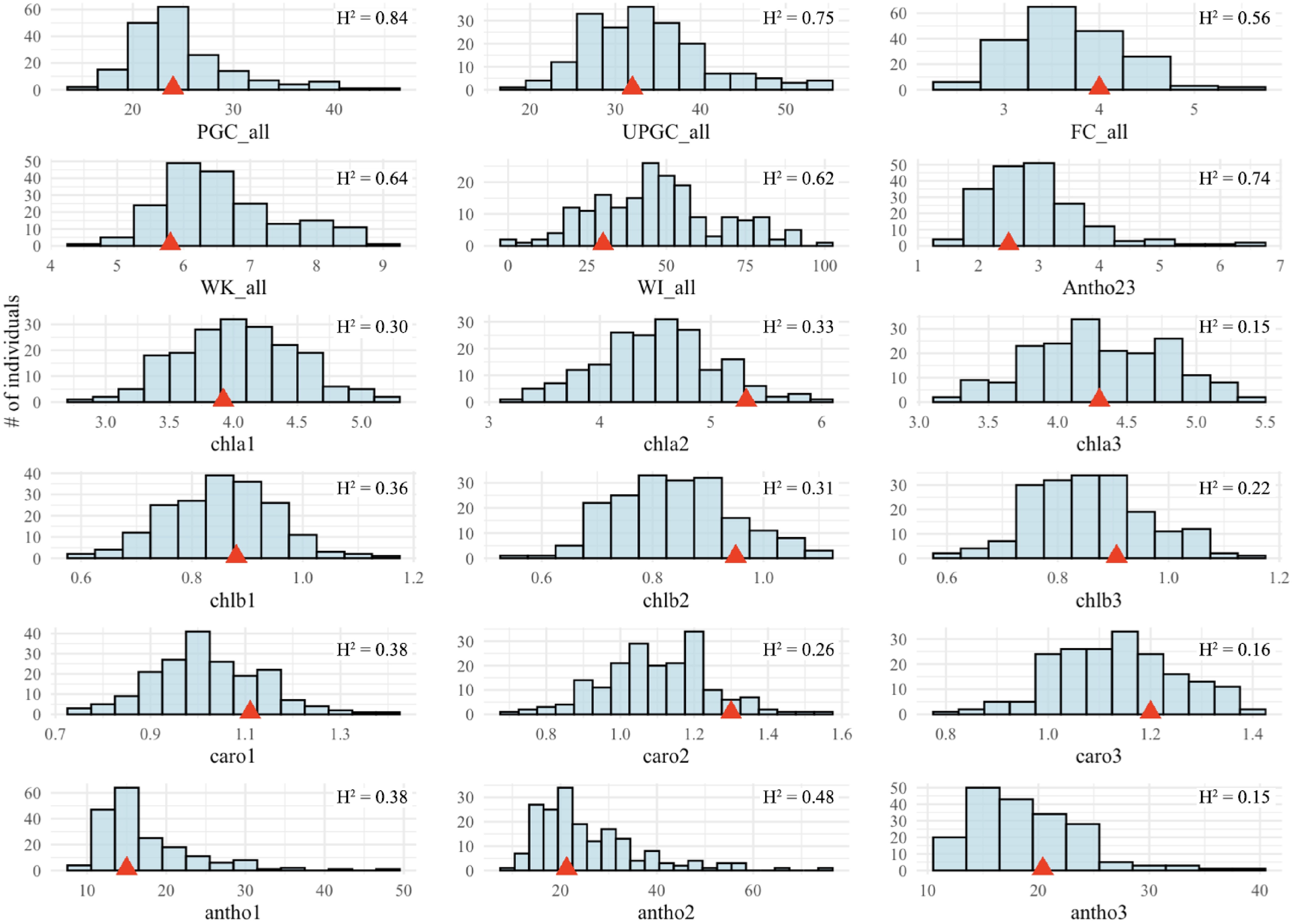
Figure 1. 

Histograms of best linear unbiased predictions (BLUEs) for winter survival traits in St. Augustinegrass Raleigh selfing population. The red triangle indicates the value for cultivar Raleigh. H² = heritability, PGC = Percent green cover, UPGC = UAS-derived percentage green cover, FC = fall color, WI = winter injury, WK = winterkill, Antho = anthocyanin rating, chla = chlorophyll a, chlb = chlorophyll b, caro = carotenoids, antho = lab-assayed anthocyanin. The '_all' indicates traits across three years, while postpositive numbers 1, 2, and 3 indicate sample collection dates on September 21, September 28, and October 12, 2023, respectively.

Pearson correlations among traits revealed distinct patterns across different years (Fig. 2). A positive correlation (p < 0.05) between winter injury and winterkill (r = 0.85 − 0.99) and between PGC and UPGC (r = 0.5 − 0.83) was observed in all three years. In 2021, positive correlations (p < 0.05) of PGC with both winter injury (r = 0.51) and winterkill (r = 0.50), as well as of UPGC with both winter injury (r = 0.37) and winterkill (r = 0.36) were observed. A negative correlation (p < 0.05) of fall color with winter injury (r = −0.49, −0.31), winterkill (r = −0.48, −0.31), and UPGC (r = −0.18, −0.21) was observed in the years 2021 and 2022, respectively. However, the correlation of fall color with PGC (r = 0.70) and UPGC (r = 0.75) was positive (p < 0.05) in the year 2023. The leaf pigments chla, chlb, and carotenoids were positively correlated (r = 0.72 − 0.87, p < 0.05) with each other at all time points. Visually-rated anthocyanin (Antho23) had a positive correlation (r = 0.39 − 0.55, p < 0.05) with lab-assayed anthocyanin at all time points. Significant positive correlation (p < 0.05) between the same traits across all three years was found for PGC (r = 0.49 − 0.55), UPGC (r = 0.24 − 0.49), WI (r = 0.20 − 0.34), and WK (r = 0.22 − 0.31). Fall color, however, had only a significant positive correlation (r = 0.48, p < 0.05) between years 2021 and 2022.

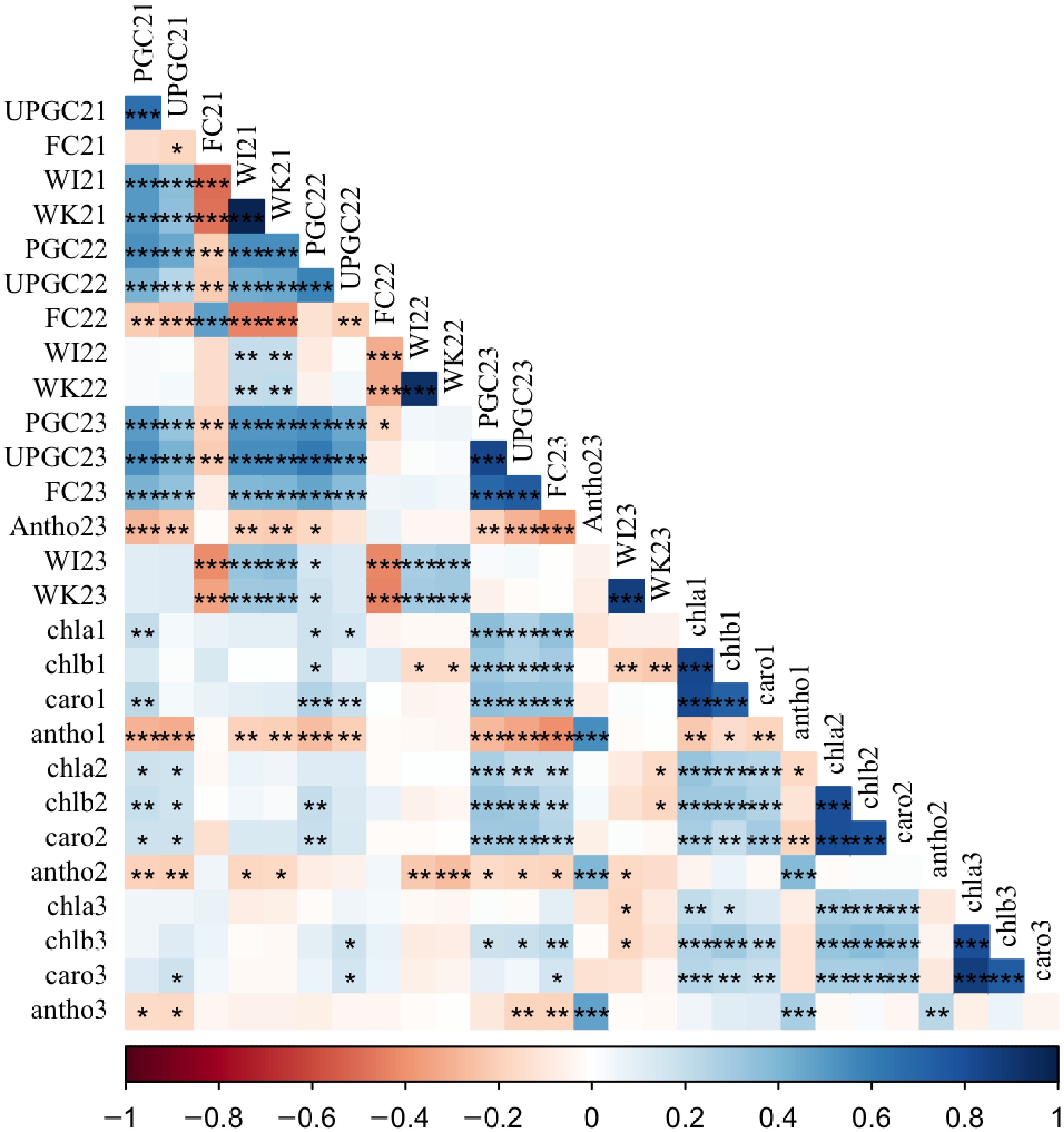
Figure 2. 

Pearson correlation coefficients for winter survival traits in a St. Augustinegrass Raleigh selfing population evaluated in 2021, 2022, and 2023 field trials and lab-assays. PGC = Percent green cover, UPGC = UAS-derived percent green cover, FC = fall color, WI = winter injury, WK = winterkill, Antho = anthocyanin rating, chla = chlorophyll a, chlb = chlorophyll b, caro = carotenoids, antho = lab-assayed anthocyanin. The 21, 22, 23, and _all on the trait column indicate years 2021, 2022, 2023, and across three years, whereas 1, 2, and 3 indicate sample collection dates September 21, September 28, and October 12, 2023, respectively. ***, **, and * indicate significance at 0.001, 0.01, and 0.05 probability levels, respectively.

Linkage mapping

Among 11,304 SNPs obtained using the GBS-SNP-CROP pipeline, 31.8% (3,593) were heterozygous in parent Raleigh. After filtering out segregation-distorted markers from heterozygous SNP markers, 2,212 high quality SNPs were retained in the final linkage map (Fig. 3, Table 1). The genome-based final linkage map contained nine linkage groups (LGs) covering a distance of 2,189.6 cM. Linkage groups 7 (184.28 cM) and 2 (315.96 cM) covered the shortest and the longest length, respectively (Table 1). The total number of markers in each linkage group ranged from 180 to 337, with the fewest markers in LG6 (180) and LG8 (180) and the highest in LG9 (337). The max gap in each linkage group spanned from 11.88 cM (LG8) to 7.35 cM (LG6), with average of 9.9 cM (Table 1). Overall, the synteny between markers on the chromosomes and markers on the linkage groups was strong (Supplementary Fig. S3).

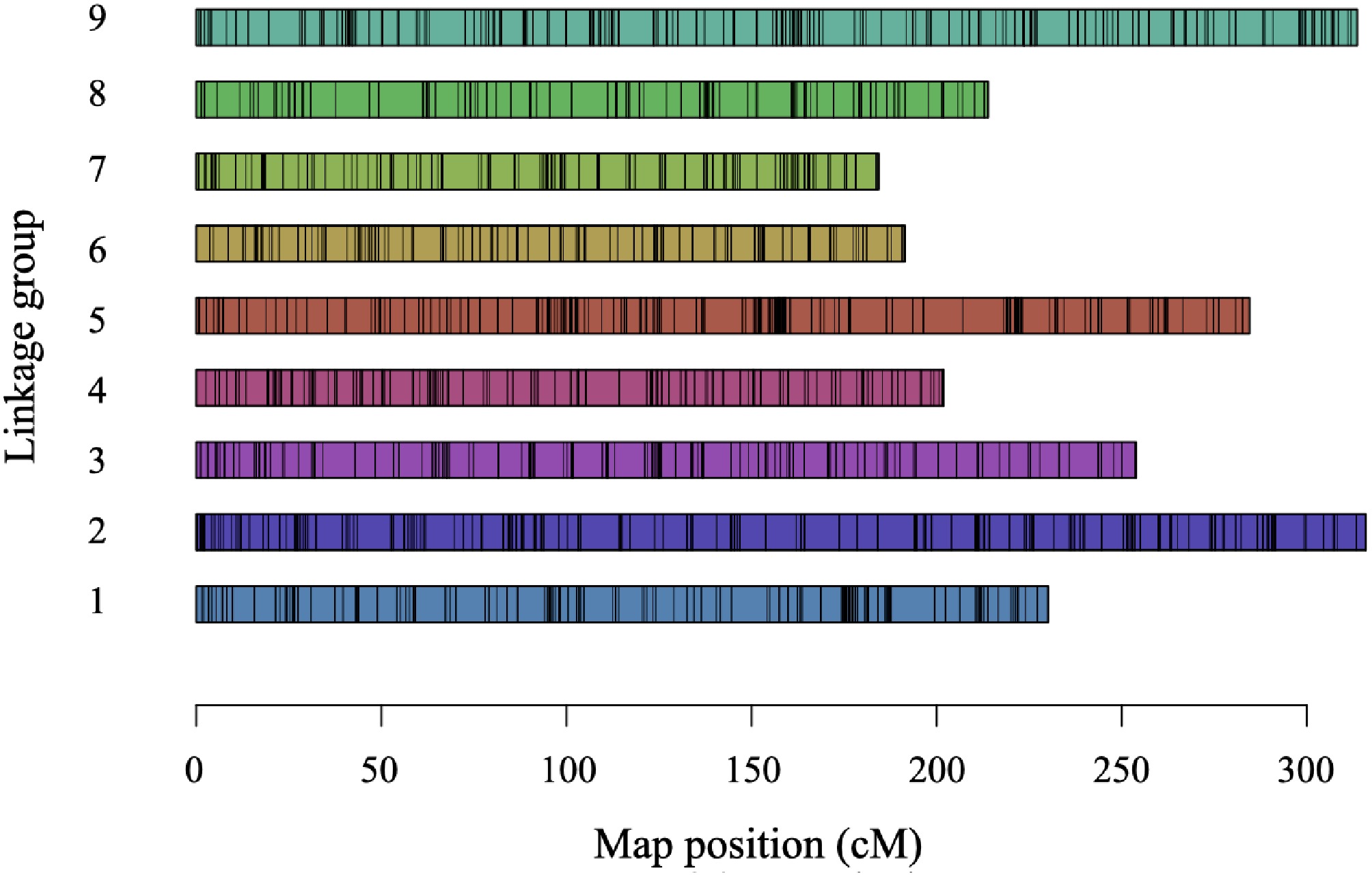
Figure 3. 

Single-nucleotide polymorphism (SNP)-based linkage map generated for a St. Augustinegrass Raleigh selfing population. cM = centimorgan.

Identification of winter survival QTL

A total of 85 QTL across all nine linkage groups were detected for all traits based on single-year and joint analysis across all three years (Table 2). The joint QTL analysis of five field-evaluated traits (PGC_all, UPGC_all, FC_all, WI_all, WK_all) across three years revealed 20 QTL across all linkage groups except LG4. The single-year analysis of field-evaluated traits for 2021, 2022, and 2023 showed 21, 11, and 23 QTL, respectively (Table 2). In addition, the single time point analysis of the lab assay leaf pigments in 2023 revealed a total of ten QTL (Table 2).

For PGC, 19 QTL were detected, with four across years, five in 2021, six in 2022, and four in 2023. Notably, overlapping QTL from at least two single years or single years and across years were located on LG3 and LG9. For UPGC, 15 QTL were detected, with five across years, two in 2021, two in 2022, and six in 2023. Overlapping QTL for UPGC were observed in LG3, LG5, LG7, and LG9. In the case of WI, 12 QTL were identified: four across years, five in 2021, and three in 2023. Overlapping QTL for WI were detected on LG1, LG2, and LG5. However, no QTL was identified for WI in 2022. Twelve QTL were detected for WK, including five across years, five in 2021, and two in 2023, with overlapping QTL found on LG5. Like WI, no QTL were detected for WK in 2022. For FC, thirteen QTL were identified, with two across years, four in 2021, three in 2022, and four in 2023. Overlapping QTL for fall color were detected on LG3 and LG9. Four QTL were detected for antho23, which was evaluated only in 2023. Lab assayed chla, chlb, caro, and antho revealed one, four, one, and four QTL, respectively.

QTL for WI and WK, the two most important winter survival traits, overlapped with QTL for other traits across several linkage groups (Table 2). Key QTL clusters, containing QTL for one or both of these traits, were identified in LG1, LG2, LG3, LG5, LG8, and LG9 (Table 2). Notably, a cluster of QTL for seven traits: WI, WK, PGC, UPGC, FC, Antho23, and antho, was discovered in LG5 (Table 2). Additional overlapping regions were found in LG1 for WI, WK, and antho; WI and antho23; and WI, WK, and UPGC; in LG2 for WI, WK, PGC, chla, and chlb; in LG3 for WK, PGC, UPGC, and FC; in LG8 for WK and Antho23; and LG9 for WI, PGC, UPGC, and FC. Multiple overlaps were also found in LG1 for WI, WK, and antho; WI and antho23; and WI, WK, and UPGC (Table 2).

Comparison with previous QTL

Eight overlapping regions were found between this study and a previous freeze tolerance QTL mapping study on the Raleigh × Seville bi-parental mapping population by Kimball et al.^[13]. WK21_1_39.61, WI_all_1_39.61, and WI21_1_39.61colocalized with RG4NCA-1 on LG1; WI_all_1_39.61, WI21_1_39.61, and Antho23_1_136.38colocalized with RG3CA-3^[13] also on LG1; WI_all_2.1_93.25, and WI23_2.2_265.09 overlapped with SGT4CA-1 and RG3CA-1^[13] on LG2; FC_all_3_200.42, UPGC_all_3_151.83, WK21_3_153.75, UPGC23_3_153.75, PGC21_3_157.76, PGC_all_3_151.83, FC23_3_151.83, PGC23_3_219.58, PGC22_3_153.75 colocalized with WK-2 (all_env), SGU-1 (all_env), SGU-1 (LW2013) and RG4CA-1^[13] on LG3; Antho23_6_99.16, PGC21_6_34.57, and Antho1_6_86.51colocalized with SGT3NCA-1, SGT4-1, and SGTNCA-2 on LG6; Antho23_6_99.16 colocalized with RG3CA-2 also on LG6, Antho23_8_210.16 colocalized with RG3NCA-2 on LG8; PGC23_9.1_10.68, FC23_9.1_13.94, UPGC23_9.1_10.68, UPGC_all_9.1_10.68, FC21_9_28.57, PGC_all_9.1_10.68, PGC22_9.1_27.86, and WI21_9_28.57 colocalized with WK-1 for single year (LW2015) and across years (all env) on LG9 (Table 3).

We also compared the winter survival QTL against drought tolerance QTL previously reported in St. Augustinegrass^[43]. Most notably, three overlapping QTL on LG3, LG6, and LG9 were found in all three studies, which showed remarkable stability across different genetic backgrounds and environments (Table 3). FC_all_3_200.42, UPGC_all_3_151.83, WK21_3_153.75, UPGC23_3_153.75, PGC21_3_157.76, PGC_all_3_151.83, FC23_3_151.83, PGC23_3_219.58, and PGC22_3_153.75 colocalized with WK-2, SGU-1, SGU-1, and RG4CA-1^[13] and PR-3.1, PR-3.2, PGC-3.2, and RWC-3.1^[43] on LG3; Antho23_6_99.16, colocalized with RG3CA-2^[13], and LW-6.1^[43] on LG6; PGC23_9.1_10.68, FC23_9.1_13.94, UPGC_all_9.1_10.68, FC21_9_28.57, PGC_all_9.1_10.68, PGC22_9.1_27.86, and WI21_9_28.57 colocalized with WK-1^[13], and AULWC-9.1^[43] on LG9.

We subsequently searched for candidate genes within the identified overlapping regions using the recently published St. Augustinegrass genome information^[39]. We found several genes involved in cold stress response via pathways including photoreceptors and light-regulation, transcription factor, calcium signaling, ROS detoxification and redox homeostasis, heat shock proteins, membrane transporters, cell wall modifiers, and photosynthesis stability (Supplementary Table S4).

Low temperature stress during the winter is one of the major abiotic stresses that limits the geographical distribution of St. Augustinegrass^[13,44]. Genetic control of low-temperature stress is highly complex, involving numerous genes, signaling pathways, and physiological responses^[45]. A deeper understanding of the regulatory networks involved in abiotic stress responses and specific genes controlling low-temperature response and winter survival is essential for enhancing winter survival through molecular breeding. In this context, QTL mapping is a powerful approach for identifying key genomic regions associated with winter survival^[13,24,25]. Moreover, QTL, which are consistently identified across populations and environments, are particularly valuable for fine mapping and MAS^[27]. Our study identified genomic regions associated with winter survival traits by comparing QTL identified in this study with those previously identified by Kimball et al.^[13] using a different mapping population and experimental trials. Within these overlapping regions, we also found potential candidate genes that could be used as target genes for improving winter survival through MAS. Furthermore, we explored overlapping genomic regions between winter survival and drought stress-related traits to identify shared genetic architecture and response pathways for adaptation to these environmental stresses^[46]. This approach also offered the advantage of narrowing down confidence intervals associated with QTL, thereby enhancing precision for MAS and the identification of candidate genes^[47]. This direct cross-validation of genomic regions between different mapping populations and abiotic stresses was enabled by the recent availability of a St. Augustinegrass reference genome^[39], which provided standard genomic coordinates by aligning QTL from different studies to a common reference.

Our study evaluated phenotypic traits PGC, UPGC, fall color, winter injury, and winterkill, over three consecutive years and found genotype by environment interaction was a significant factor for all these traits. The correlation of the same or different traits varied between years in our study, further supporting the presence of genotype-by-environment interactions and the strong influence of environments on low-temperature response. This could present a challenge in pinpointing reliable QTL across environments by detecting unique QTL in different years due to varying environmental conditions^[25]. We found numerous non-overlapping QTL for the same or different traits within and between years. This could partially be explained by the presence of no to low correlation between them and the complex genetic control of these traits^[25]. By identifying QTL for single-year and joint analysis across three years and comparing them, we accounted for these interactions within our study, too. We also incorporated physiological traits (chlorophyll a, chlorophyll b, carotenoids, and anthocyanins) known to support cold acclimation, winter dormancy, and winter survival in turfgrass^[17,19]. Additionally, our study introduced Antho23, a visual rating for anthocyanin-based reddish/purplish pigment development in the fall for the first time. We found QTL overlap among multiple winter survival traits, suggesting pleiotropy and/or genetic linkage between the genes controlling those traits and indicating a shared genetic basis for these traits^[48]. Overlapping of QTL associated with multiple traits also narrowed down the genomic regions of interest, facilitating candidate gene identification for further investigation. While identifying pleiotropy and genetic linkage was beyond the scope of our study, differentiating the underlying mechanisms between them in future studies could provide breeders with valuable insights into target genes to improve multiple traits simultaneously^[49].

Only 31.8% (3,593) of the SNPs detected in our study were polymorphic for parent Raleigh, which significantly reduced the initial number of markers available for linkage map construction. However, 2,212 segregating SNPs were included in the final linkage map. In comparison, Kimball et al.^[13] used SSR markers with patterns homozygous for one parent and heterozygous for another or heterozygous for both parents in a Raleigh x Seville biparental population. The heterozygous SNP markers identified in our study complement the heterozygous SSR markers for parent Raleigh^[13]. The linkage established in our selfing population relied on only a single cycle of meiosis, resulting in lower recombination events and high linkage disequilibrium. While high linkage disequilibrium facilitated QTL detection even with a low-density linkage map, it is important to note that the limited recombination events and high linkage disequilibrium likely resulted in the identification of large QTL, which presented a challenge in detecting QTL with high resolution^[25,50,51]. Despite these limitations, our study identified eight overlapping regions across chromosomes 1, 2, 3, 6, 8, and 9 that aligned with the previous winter survival QTL in the Raleigh × Seville mapping population^[13]. QTL identified for winterkill, the only trait evaluated in both studies, overlapped on chromosome 9. A single year and across year QTL associated with PGC, UPGC, fall color, and winterkill overlapped in this region, which had the second highest (eight) number of QTL overlaps in our study. In addition, overlapped QTL on chromosome 3 contained both field and laboratory-based/controlled environment testing from Kimball et al.^[13] and single and across-year QTL from our study. These results suggest a strong association of these regions for the genetic control of winter survival in St. Augustinegrass, making them prime targets for developing MAS.

Identifying candidate genes within regions of overlap and validating their function is crucial because it helps pinpoint genes with functional mutations that contribute significantly to trait variation^[52]. Within the overlapping regions identified, multiple candidate proteins with a wide range of molecular functions and biological processes were found to be involved in low-temperature stress response (Supplementary Table S4). Here are several example candidate genes. F-box with LRR domain was identified on chromosome 1, which is associated with response to abiotic stress, particularly through abscisic acid signaling, and is known to be expressed under cold acclimation and stress in soybean (Glycine max [L.] Merr.) and Arabidopsis (Arabidopsis thaliana [L.] Heynh.)^[53,54]. Two genes encoding Zinc finger CCCH domain-containing protein were identified on chromosomes 1 and 6. In transgenic switchgrass (Panicum virgatum L.) cold-induced expression of the CCCH zinc-finger protein PvC3H72 led to improved cold tolerance, higher survival rates, relative water content, and stable cell membranes by regulating the ICE1-CBF-COR complex and abscisic acid pathway genes^[55]. The genes encoding Zinc finger CCCH domain-containing protein have already been identified as a potential candidate gene for winter survival in zoysiagrass^[56]. In chromosome 2, WRKY transcription factor WRKY62, which is involved in abiotic and biotic stress tolerance through a complex network of salicylic and/or jasmonic acid-mediated signaling pathways^[57] was annotated. Our study identified SWEET11, a bidirectional sugar transporter which facilitates sugar movement across cell membranes in response to abiotic stress, including cold and drought stress^[58,59]on chromosome 3. Additionally, Arabidopsis SWEET11 and SWEET12 mutants have shown increased freezing tolerance compared to wild-type plants, further supportifng the role of SWEET transporters in cold stress adaptation^[60]. All these genes are promising candidates for MAS implementation, however, their functions in St. Augustinegrass need to be validated in future studies.

In summary, the QTL identified in this study along with the comparison with previous studies, revealed overlapping genomic regions. Associated markers have the potential to be used in breeding and selection of St. Augustinegrass for enhanced winter survival. The candidate genes/proteins identified in this study also could be valuable additions to St. Augustinegrass breeding programs. These proteins contributed to crucial molecular functions and cellular processes, highlighting the complex genetic architecture of low-temperature stress. Examining their combined effects will deepen our understanding of the genetic response to low-temperature stress and underlying tolerance mechanisms. These findings not only solidify the role of these genes in winter survival but also support their application in MAS to develop stress-resilient St. Augustinegrass cultivars with broader adaptation.