A comparison of state-of-the-art reinforcement learning algorithms applied to the traveling salesman problem

This paper compares the performance of a variety of RL algorithms on the Traveling Salesman problem (TSP), and the Orienteering Problem (OP), and examines their generalization capabilities with regard to problem instances of untrained sizes. In the following, the two core concepts of combinatorial optimization problems, and RL solution algorithms with the capability to generalizd are introduced and motivated. The contributions of this paper, as well as its structure is summarized in section "Contributions".

1.1.   Combinatorial optimization problems

Combinatorial optimization problems are mathematical optimization tasks that involve selecting a subset from a finite set of discrete elements such that it maximizes or minimizes a specific metric under given constraints. A famous example of such a combinatorial optimization problem is the knapsack problem. The goal is to select a subset of items that have sizes and values such that a knapsack with limited capacity can be filled to a maximal value. Combinatorial optimization problems like this have significant implications for real-life use cases. Solutions to the knapsack problem, for example, can be used to improve transportation by maximizing value in deliveries with limited capacity, to improve inventory management by deciding which items to keep in a warehouse of fixed size, or to determine what data streams to prefer in limited bandwidth applications. This paper focuses on the two combinatorial optimization problems: the Traveling Salesman Problem (TSP), and the Orienteering Problem (OP), which will be introduced in detail in subsequent sections.

1.1.1.   Traveling salesman problem (TSP)

The TSP is traditionally a graph combinatorial optimization problem, where a fully-connected graph with edge weights and n nodes is considered. The objective of the TSP is to find a minimum Hamiltonian cycle, i.e., a closed-loop in the graph that visits each node exactly once and returns to the initial node with the smallest possible cumulative edge weight. A subset of all TSP instances can also be represented as metric problems, where instead of a graph, node coordinates are given, and all of the distances are inferred based on the metric distances. Popular optimal solvers for TSP are Concorde (see Applegate et al.^[1]), and the general-purpose solver Gurobi^[2]. The TSP is NP-hard^[3], which means optimal solvers may have exponential time complexity and, in general, do not scale well with the problem size.

For approaching larger TSP instances, several heuristics have been developed^[4], but they may only achieve satisfactory results on specific distributions of problem instances, cf.^[5]. In the real world, the TSP has applications in delivery planning, for example, where better solutions can lead to significant benefits in time efficiency and environmental sustainability. See examples of practical variants of TSP in the citations here^[6−10].

1.1.2.   Orienteering problem (OP)

The second combinatorial optimization problem covered by this article is the OP^[11]. Like the TSP, the OP is also originally a graph combinatorial optimization problem based on fully-connected graphs with edge weights. In addition to that, OP instances incorporate a depot node, a range value, and node values that can be considered prizes. The objective in the OP is to find a tour that maximizes the cumulative prizes of the visited nodes while starting and ending at the depot node, with cumulative edge weights smaller than or equal to the given range value. As for the TSP, metric problem definitions exist for the OP. The OP is also referred to as the Generalized Traveling Salesman Problem^[12], and is proven to be NP-hard as it contains the TSP as a particular case^[11]. The Gurobi optimization suite, and the RB & C TSP solver, cf.^[13], are examples for algorithms that can solve OP instances optimally. The Compass algorithm, cf.^[14], is an example of a heuristic approximator for solutions to the OP. As the name implies, the OP can be used in the real world to optimize orienteering in an unknown environment. Exploration like this could be carried out by humans within a limited time, representing the range value in this case. It could also be performed by a drone, for example, with a range limited by the battery size.

Calculating exact solutions to combinatorial optimization problems is often challenging because many of those problems are NP-hard, i.e., solutions in polynomial time are not known. Therefore, all optimal solvers have at least an exponential time complexity, making them less applicable for large problem instances. Because of this, sizeable combinatorial optimization problem instances are usually approached by complex, expert-crafted heuristics and approximations. In recent years, RL has gained popularity and is promising to become a powerful alternative or extension to expert-crafted solutions, especially due to the possibility of applying trained agents to untrained problem sizes.

1.2.   Generalizing solutions using reinforcement learning (RL)

RL is a field of machine learning concerned with training a machine learning model (cf. agent) to take actions in a Markov decision process (cf. environment)^[15] based on observations of the environment's state to maximize the expected, cumulative discounted rewards. The idea of RL has been around since the 1950s, but received a surge in popularity in 2013 when researchers of DeepMind demonstrated an algorithm that could learn most of the Atari games from scratch. This algorithm was called Deep Q-Learning (DQN), and will also be covered in this paper. Since then, various RL algorithms and extensions have been developed for all kinds of applications.

In this paper, RL will be applied and compared to the combinatorial optimization problems TSP and OP. In the future, breakthroughs in this direction could drastically reduce carbon emissions by optimizing transportation chains, for example. As an alternative to RL, supervised learning requires expensive, optimal solutions for learning to approximate combinatorial optimization problems and would effectively learn to replicate the optimal solver used to generate the training data. In addition, there might be multiple optimal solutions to single problem instances, which the model would only be aware of if it were trained on many of them. RL is a promising approach as it only requires a suitable reward function, and some training data. Over the training process, the model incrementally builds better solutions by itself, and has the capability to provide out-of-the-box solutions for unseen problem instances. Downsides of RL are the opaque selection of algorithms and their extensions, and the more complicated tuning compared to Supervised Learning. In contrast, the sequential solution generation of RL algorithms entails unique generalization capabilities with respect to problem sizes.

1.3.   Contributions

Most RL research just presents a single RL approach without detailed information on why a particular algorithm was chosen. Additionally, even though the generalization capabilities of RL for combinatorial optimization problems have been mentioned in other sources, the topic has not been covered in detail. The main goal of this paper is to give a comparison of multiple RL algorithms on the TSP and OP, and to examine their generalization capabilities while giving possible reasons for the observable differences.

The main contributions of this paper are the following.

(1) The performance of state-of-the-art RL algorithms are studied and compared when applied to the TSP and the OP, which have the capabilities to generalize, i.e., after pretraining, are able to provide fast out-of-the-box solutions for unseen problem instances.

(2) The tuning of selected RL algorithms are optimized and their performance compared on the TSP and OP with existing RL combinatorial approximators as well as optimal solver-based solutions (for single tractable problem sizes).

(3) Further, the quality of their generalization capabilities regarding the problem size, i.e., when applied to larger problem sizes that have not been seen in training, are analyzed.

As optimal solver-based approaches for the TSP do not scale well for larger problem instances, heuristic solutions are required. In this context, e.g., divide-and-conquer methods have been used to solve the TSP in a decoupled fashion^[16,17]. In this line, to cluster nodes within a close region, more recent approaches use, for example, grid-based methods^[18,19], density clustering^[20], or k-means clustering^[21].

Another stream of research uses further ML techniques to approach TSP problems^[5,22,23]. Various papers propose heuristics for the TSP by using, for example, specific model architectures^[24,25], learning paradigms^[26−28], graph networks^[29−31], and genetic algorithms^[32,33].

Most of the works mentioned above are limited to small-scale TSP with, at most, 100 nodes. Although the generalization capabilities of some models make them applicable to instances of larger scale, their performance drops significantly with an increasing number of nodes.

While there exist many different approaches to (approximately) solve small or extremely large TSP problems for a fixed instance, algorithms that generalize and, after pretraining, allow to heuristically solve different problem instances have been much less studied.

The paper that is closest to the present is the study by Kool et al.^[27]. The authors use a vanilla REINFORCE RL algorithm with their greedy rollout baseline. They show that pretrained models can generalize and heuristically solve TSP problem instances with altered input. The studied problem sizes range from 20 to 100 nodes. The quality of their solutions has been compared against previous work by Bello et al.^[26] and Dai et al.^[30], which is mentioned in Table 1.

While Kool et al.^[27], experiment with different baselines, and apply their solutions to a few additional combinatorial optimization problems, the article lacks a comparison to other RL approaches. The capability to generalize to larger problems than seen in training is mentioned in the Supplementary File 1, but not studied in detail.

RL algorithms and suitable ML architectures for combinatorial optimization problems are promising tools for that kind of problem. However, in this context, the performance of different RL algorithms is unclear. The goal of the present study is to close that gap. Particularly, the case in which a generalizing model is used to address problems that are larger than the model has been trained on, and is less well researched.

2.2.   State-of-the-art RL algorithms

This section introduces some of the most popular RL algorithms, which will be considered in the present experiments. In Section "Evaluation and performance comparison", these RL algorithms will be tuned, evaluated, and compared on the combinatorial optimization problems TSP and OP.

2.2.1.   Q-learning and deep Q-learning (DQN)

Q-Learning, cf.^[34], is used for decision processes with potentially infinite horizons, finite action, and state spaces, but imperfect information regarding state transition probabilities and reward functions. The algorithm learns the expected future rewards of all state-action pairs (Q-values) to compensate for the imperfect information. This way, a policy can be defined by taking the actions with the largest Q-values. The decision process is explored similarly to approximate Dynamic Programming taking actions based on the current iteration of the policy with $ \epsilon $-greedy decisions. The Q-values are often initialized randomly and updated gradually with each step using the learning rate α $ \in $ (0, 1), as the missing transition probabilities prevent the explicit calculation of expected values.

Q-Learning can only be applied to single instances of TSP or OP because every instance has a finite horizon, a finite action, and state-space, and all state transition probabilities and corresponding rewards are known. However, the state spaces of these instances have factorial complexity, and the algorithms above might fail due to memory limitations, especially for larger program sizes.

In addition, Q-Learning cannot produce a general policy that can be applied to any TSP or OP instance of a specific size. The general case of e.g., 20 nodes, has an uncountable state set, as the edge weights or node coordinates are continuous. Deep Q-Learning, cf. Deep Q-Networks (DQN)^[35,36], solves both issues by replacing the Q-value table with a regression algorithm, typically a neural network. Several extensions and improvements to the Deep Q-Learning approach have been developed. Double Deep Q-Networks (DDQN)^[37], derived from Double Q-Learning, cf.^[38], introduces a second neural network, and updates each neural network with a bootstrapping value of the opposite. This reduces overestimation bias, which occurs when too-high initialized Q-values are explored and used for bootstrapping. This way, biased estimates are backpropagated, and without DDQN, it can take a long time until the network unlearns this bias.

2.2.2.   Policy gradient (PG) variants

All of the following algorithms include some form of policy optimization. Instead of only learning the expected future return of states and state-action pairs, and implicitly learning a policy, policy optimization methods directly learn a distribution over all actions, explicitly defining a policy that tries to maximize the expected future return.

Policy Gradient (PG)^[39−41], is a family of policy optimization algorithms that reinforces the probabilities of taking actions based on some performance metric. Which kind of metric is used has significant implications for the bias-variance trade-off of the gradient calculation. One of the simplest PG algorithms, referred to as vanilla PG, cf.^[42], increases the probabilities of actions proportional to the total (discounted) reward of their respective trajectories, which results in a high variance of the gradient approximations for two reasons. Actions are reinforced based on rewards of preceding actions, and depending on the reward function, probabilities are potentially only ever increased and never decreased explicitly.

REINFORCE^[43], is a popular PG algorithm that improves on the vanilla variant by reinforcing actions based on their realized (Monte Carlo) reward-to-go. More advanced PG algorithms subtract a state-dependent baseline value from the reward-to-go, isolating the advantage score of the actions, and reducing the gradient approximation variance by removing the expected return in a state from the reinforcing term.

2.2.3.   Advantage actor-critic (A2C)

Actor-critic algorithms are also policy optimization methods like the PG variants. In addition, they also include some form of value-learning, as described in the Deep Q-Learning section, for estimating at least one of the state-values or state-action-values. In the case of the Advantage Actor-Critic algorithm^[44], at least one state-action-value learner, called a critic, is implemented to calculate advantage-values for each action.

A popular extension of A2C is A3C, Asynchronous Advantage Actor-Critic, cf.^[44]. In this variant, multiple actors and critics are trained in parallel, and actors are synced independently and periodically with global parameters.

2.2.4.   Proximal policy optimization (PPO)

Catastrophic forgetting, in the form of high training instability, is a common problem with RL algorithms, cf.^[45]. Especially policies learned by policy optimization methods can drastically change between single updates, causing insufficient exploration, and taking many iterations to recover. Proximal Policy Optimization, cf.^[46], is another actor-critic variant designed to reduce this issue by limiting the changes to the policy in-between updates. This is achieved by either the PPO-Penalty or the PPO-Clip method. PPO-Penalty includes a KL divergence term of the old and the new policy in the objective function and adjusts the penalty coefficient throughout training. PPO-Clip is the method implemented in this article. It introduces a unique value-clipping mechanism to the loss function, removing the incentive of the new policy to move far away from the previous, fixed policy.

2.2.5.   Soft actor-critic (SAC)

The main feature of the Soft Actor-Critic algorithm, cf.^[47], is entropy regularization. The entropy of a discrete random variable quantifies the amount of 'surprise' in the variable's possible outcomes. The entropy is largest when all possible outcomes have the same probability. SAC aims to learn a policy that maximizes the expected future return while acting as randomly as possible, i. e., keeping the probability distributions over the actions as flat as possible and, therefore, having a high entropy. To do this, an entropy term is included in the Q-learning objective, which gives it the name soft Q-learning. Haarnoja et al.^[48] also describe the possibility of learning the entropy temperature parameter α. The idea behind SAC entropy temperature learning is to learn a value that adjusts the expected entropy over all decisions of the policy towards a desired value. This way, the policy is allowed to have low entropy in some states, where specific actions are clearly advantageous. Based on SAC, further variants exist, e.g., distributional SAC^[49].

2.3.   Related machine learning concepts and architectures

The approximation of solutions to combinatorial optimization problems benefits from neural network architectures with unique properties like input permutation invariance, and the ability to process instances in graph representation or of varying problem sizes. This section introduces the most important concepts and architectures for approximating combinatorial optimization solutions.

2.3.1.   Attention and transformers

Attention in machine learning^[50] is a mechanism that enables a neural network to learn how to combine multiple data points in a meaningful way. Attention is widely used to establish global awareness for variable-length sequences or order-invariant inputs. Each attention calculation involves a query vector, and n–1 key, and value vectors. The compatibility of the query vector with each of the key vectors can be determined using dot product calculations. The softmax operator is applied over all n–1 (optionally scaled and masked) compatibility scores to produce attention weights between 0 and 1. The output vector of this single attention run is a sum of the value vectors, weighted by the corresponding attention weights. Usually, n attention runs are executed with each input once as a query to produce n output vectors, one for each input. The neural network can learn how much each input should attend to each other input by learning the query, key, and value embeddings using preceding transformations like MLPs. In multi-head attention (MHA) layers^[51], the n attention runs, including preceding transformations, are executed m times, resulting in m different embeddings for each input, which are then aggregated. This allows the network to learn and combine multiple attention patterns.

Similar to recurrent neural networks (RNNs), transformers^[51] consist of an encoder and a decoder, and can produce variable-sized outputs to variable-sized inputs. Instead of implementing traditional RNN architectures, like LSTMs^[52], transformers are originally based on attention mechanisms. A possible architecture of a transformer network is depicted in Fig. 1a.

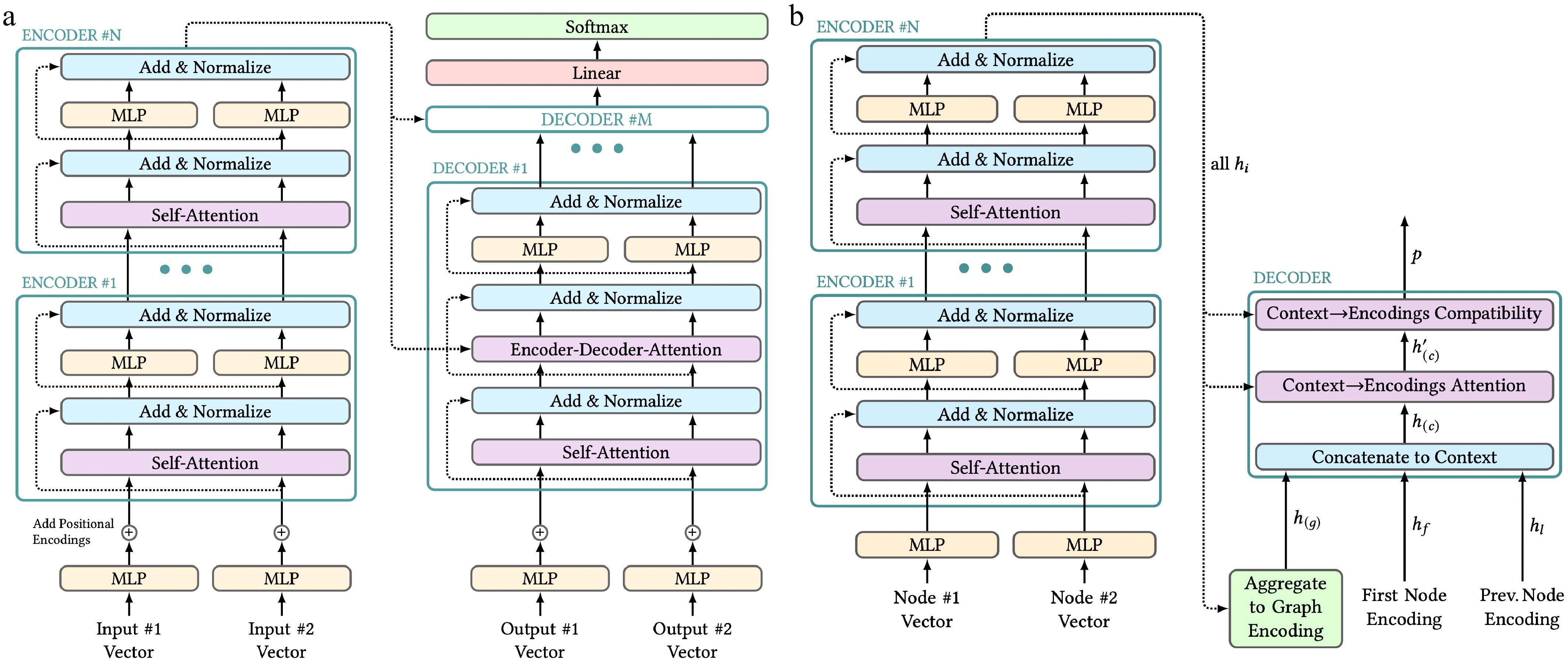
Figure 1. 

Transformer architectures. Figure style adapted from Alammar^[53]. (a) Structure of a transformer proposed by Vaswani et al.^[51] with two representative input vectors on both sides. In practice, any number of inputs can be passed to the encoders and decoders. (b) Structure of Kool, Van Hoof, and Welling's transformer for approximating solutions to the Traveling Salesman Problem.

The encoder side consists of a small preprocessing unit, followed by a sequence of N architecturally identical encoder layers. The preprocessing unit embeds each input element using a shared, learnable transformation. This could be a multi-layer perceptron (MLP), for example. For sequence tasks, each of the embeddings is extended with a positional encoding before being passed to the sequence of encoder layers. Each layer consists of a multi-head attention mechanism, followed by another shared, learnable transformation. Feedforward connections, combined with normalization, prevent loss of per-node information and numerical overflows. The final outputs of the last encoder layer, which are embeddings of the input vectors, are passed to each of the decoders.

The architecture on the decoder's side is similar to the encoder. In each decoding step, the previous outputs are embedded by a preprocessing unit and optionally receive a positional encoding before being passed into a sequence of architecturally identical decoder layers. In each layer, a multi-head self-attention mechanism is applied to all the output embeddings first, followed by a joint multi-head-attention operation of all the input and previous output embeddings. Queries for this 'Encoder-Decoder-Attention' block are only generated from the embeddings of the outputs. If a decoder receives n input embeddings, and m output embeddings, its output will be of size m. During the training phase, the whole desired output sequence can be fed into the decoder, which will predict the succeeding item for each position. The 'Encoder-Decoder-Attention' block contains masking operations to prevent the decoder from just learning to copy the following items from the input by attending to future elements of the sequence. Each decoder layer also includes a shared, learnable transformation. After all those layers are finished with calculations, the final embeddings are passed through a linear transformation, and output probabilities can be generated using the softmax function.

2.3.2.   Metric combinatorial approximators

With the development of Pointer Networks in 2015, Vinyals et al.^[25], initiate the research towards metric combinatorial approximators. Bello et al.^[26] advance the work of Vinyals et al.^[25] by using Pointer Networks with an RL approach to approximate metric TSP solutions. Their RNN encoder-decoder architecture consists of Long Short-Term Memory (LSTM)^[52] cells. The encoder sequentially processes the input elements and generates an encoding of each input enc_i. Similarly, the decoder processes the hidden state of the previous execution as well as the last action to produce an output vector dec_j in each decoding step. An attention mechanism determines the following action using all enc_i and the last dec_j. Bello et al.^[26] train this Pointer Network using an RL setup related to A3C.

Nazari et al.^[54] point out two limitations of the work by Bello et al.^[26]. An LSTM encoder, as implemented by Bello et al.^[26], produces different encodings depending on the permutation of the input elements. Permutation-invariant processing of the metric problem instances is desirable, as the optimal solutions are not permutation-dependent and training on all possible permutations is computationally infeasible.

As a solution, Nazari et al.^[54] proposes dropping the encoder and using a special RNN decoder. At each decoding step t, this unit receives the embedding of the previous action $ \bar{s}^a_{t-1} $ and all of the current nodes' features, composed of a fixed component sⁱ and a dynamic component $ d^i_t $ as inputs. At each step, $ \bar{s}^a_{t-1} $ is fed into a small LSTM cell that produces a 'memory state' h^t. Additionally, all of the node features are embedded to $ \bar{s}^i $ and $ \bar{d}^i_t $ using a shared, learnable transformation. A series of attention operations produces a probability map for the next actions: the hidden state is used as a query in a single attention operation with all other embeddings as keys, producing attention weights a_t and an aggregated context consisting of $ s_t^c $ and $ d_t^c $. The attention weights between the context and all input embeddings are calculated, producing the output probability map p_t. Nazari et al.^[54] train this RNN decoder using the A3C RL algorithm.

Kool et al.^[27] take advantage of the development of the transformer architecture^[51], by modifying it for combinatorial optimization. The encoder unit of their transformer receives all of the node features as input. In contrast to the original architecture, the node embeddings are not extended by a positional encoding, as node permutation-invariance is desired. Instead, they are passed directly into N encoding layers, consisting of MHA operations and MLPs, as described by Vaswani et al.^[51]. The encoder outputs n node embeddings and a graph embedding, which is computed as the mean of the node embeddings. The decoder includes more adjustments, as it needs to output input-sized instead of fixed-sized probability vectors. Additionally, the decoder must consider some problem-specific features for each combinatorial optimization problem.

For TSP, the decoder input consists of all the encoder node embeddings h_i, the encoder graph embedding h_(g) and the embeddings of the first and last node (h_f, h_l) of the partial solution. First, a context node is created by concatenating h_(g), h_f and h_l. This node contains all the relevant information to the current partial solution. The context node h_(c) and the encoder node embeddings h_i are passed to a multi-head attention mechanism, but only a single query from the context node is computed per head. The results are aggregated to produce a new context node embedding $ h'_{(c)} $. A final single attention query from $ h'_{(c)} $ to all the encoder node embeddings h_i is executed, resulting in a probability map p for the next action. Nodes that have already been visited are masked in these attention mechanisms.

The complete architecture is depicted in Fig. 1b. Kool et al.^[27] use this transformer to learn a stochastic policy optimized using the vanilla (full-trajectory) Policy Gradient algorithm with several baseline options. Using this setup, Kool et al.^[27] approximate metric versions of the Traveling Salesman Problem (TSP), the Orienteering Problem (OP), the Vehicle Routing Problem (VRP), and the Price-Collecting TSP (PCTSP).

Finally, Table 1 compares optimality gaps, average solution lengths, and runtimes, of related approximators^[26,27,30] on TSP instances with n = 20, 50, and 100 nodes.

In this section, the present research setup, and the optimization of RL algorithms to be compared are described. Then, we compare the solution quality of RL algorithms for the TSP, and the OP are compared.

3.1.   Setup and optimization of selected RL algorithms

How the TSP and OP are modelled as MDP to be solved via RL algorithms are first described. RL algorithms are then selected to be compared, their hyperparameter optimization for fair comparisons discussed. The present study implementations and RL frameworks used are described in Section "Setup and implementation".

3.1.1.   Applying RL algorithms to the TSP and OP

In this section, how to apply selected RL algorithms to be compared on the TSP and OP are described. The concepts and computations behind TSP and OP are fully known, which means that complete models of the problems are available, and there are no non-observable parameters. Embedded as Markov Decision Process (MDP), the state transitions are deterministic with selected actions, and reward functions are defined by edge weights, or can be calculated as distances between the nodes.

The state set (cf. state space) of single TSP and OP instances (i.e., the number of nodes) are countable, but the general problem that solves any instance of n nodes has uncountable state sets (continuous potential coordinates for all nodes). To create efficient and general approximators for TSP and OP, table-based learning approaches are not considered. All algorithms taken into consideration use neural networks for regression.

Further, the action sets for combinatorial optimization problems are all countable. This poses some restrictions to possible RL algorithms. Algorithmic adjustments are also necessary for methods like SAC, for example, as it is originally not designed to work with discrete, countable actions.

Moreover, the TSP and the OP have finite horizons, as there is a limited number of nodes per problem instance. Infinite horizon solutions can still be applied. Additionally, combinatorial optimization problems are naturally step-based and operate in discrete time.

3.1.2.   Selected variants of RL algorithms

For the comparisons in this paper, variants of the algorithms introduced previously are used. DQN is chosen to represent the value-learning algorithms. Additionally, Q-values learned with a discount factor of 1 accurately reflect the optimal solution length to-go, i.e., the reward function is well-defined. The DQN agent uses epsilon-greedy exploration. The algorithm's deterministic nature can benefit optimality, as stochastic policies do not have benefits for TSP and OP besides exploration. The DQN agent implemented is a Double DQN variant, which reduces the overestimation bias of the target values for faster learning.

The PG algorithm by Tianshou^[55], is a Monte Carlo reward-to-go PG implementation. It is included in the analysis for comparisons to the Kool et al.^[27] vanilla PG variant with baselines. In theory, it has less variance in the gradient approximations than the vanilla version without baselines. The algorithm includes exploration by the stochastic policy.

The SAC algorithm is selected as a representative for entropy-regularized RL algorithms. It learns off-policy and can have advantages in execution time, as fewer samples need to be generated. Analyzing this is not a focus of this paper, and, as previously mentioned, custom implementations should be used instead of customizable frameworks for more detailed comparisons. The benefits of entropy regularization for combinatorial optimization problems lie solely in the exploration during training. After training, surprise and unpredictability in actions are less desirable than optimal performance.

A2C and PPO are included in the experiments as successors and alternatives to the classic PG variants. These algorithms use Generalized Advantage Estimation (GAE, Schulman et al.^[39]) in the Tianshou implementation and should have a lot less variance in the gradient approximations than Monte Carlo PG methods. Still, there might be some bias introduced by the advantage approximations. PPO reduces incentives for drastic policy changes by objective function clipping. Therefore, it might be more stable and less hyperparameter sensitive than the other algorithms.

3.1.3.   Hyperparameter optimization and performance metrics

For a fair comparison, the five selected RL algorithms have to be optimized for the TSP regarding their individual hyperparameters. Note that the corresponding details are described and analyzed in the respective parts of the Supplementary File 1.

All algorithms are optimized on the 20-node TSP first and evaluated on TSP and OP in later sections of this paper. The mean length of optimal TSP solutions of 20-node metric instances (determined via solver, see additional reference values in Table 1) placed in a unit square is 3.84, and serves as a lower bound regarding the achievable mean length. The mean length of random TSP solutions of 20-node instances is 10.43, which serves as a second performance baseline.

Unless otherwise specified, every data point in the performance graphs of this paper is a mean solution over 1,280 test problem instances, achieved through deterministic evaluations of the policies.

3.1.4.   Setup and implementation

The implementation of the present experiments is based on the methods of Kool et al.^[45] (GitHub repository: https://github.com/wouterkool/attention-learn-to-route).

Kool et al.^[27] achieve state-of-the-art results for RL combinatorial optimization using a Transformer architecture and a full-trajectory PG approach. Their article lacks information on why they selected PG as their RL algorithm. Recent advancements in RL claim improvements compared to PG methods in many aspects such as exploration, optimality, stability, and convergence rate. Kool et al.^[27] also provide evaluations on multiple combinatorial optimization problems and some results on generalization to larger problem instances in the Supplementary File 1, which yields many factors for comparison.

The solutions of Kool et al.^[27] are not using any RL framework, and includes custom calculations for the PG loss. Their model is designed to receive a batch of problem instances, solved completely over multiple steps within the model. After a batch of problem instances is solved, the model returns the sum of realized rewards and the sum of log probabilities for each episode, used to calculate the loss. By this original design, all of the partial solutions in a batch of instances have the same progress, and all start entirely unsolved. Additionally, the encoder only needs to be executed once per problem instance instead of once per transition.

With the transition to a modular setup with Tianshou, the model is adjusted not to solve full episodes of problem instances, but to predict the subsequent best actions to a batch of partially-solved instances of varying progress. These changes require the execution of the encoder for every transition during training. In addition to the changes to the RL policy model, the code for the problem environments is refactored to comply with the OpenAI Gym API supported by Tianshou. All occurrences of environment observations are adjusted to handle the changed data formats correctly.

For actor-critic algorithms, the baselines implemented by Kool et al.^[27], cannot be used, as they produce reference values for whole trajectories. For the transition-based setup with Tianshou, two new critics are developed, which generate value estimations for partially solved problem instances. The v3 estimator uses an architecture almost identical to the refactored policy model, in theory making it really powerful and promising precise value-estimations. The v1 critic mainly consists of a preprocessing unit, an encoder, and a small MLP which is a more lightweight option compared to the v3 estimator. In the preprocessing unit, node features are extended by information that the policy model (and the v3 encoder) adds in the decoder part.

Besides its 2D coordinates, after preprocessing, each node of the v1 critic also contains 0/1 encoded dimensions, indicating whether it was visited already and whether the node was the first or last node of the partial solution. These node extensions are problem-specific and detailed investigations of critical architectures could be subject to future work. All of the implementation adjustments enable high modularization for detailed comparisons of different RL algorithms.

3.2.   Performance comparison for the traveling salesman problem (TSP)

This section compares the best configurations of each RL algorithm. Each agent is trained over 300 episodes on the 20-node TSP, and exponential learning rate decay is used for all algorithms, except for SAC. The decay factor is adjusted to 0.9999 for the Tianshou agents and 0.99 for the algorithm of Kool et al.^[27], which results in a very similar learning rate decay when adjusted for the update frequencies that differ by a factor of 100 (0.9999¹⁰⁰ ≈ 0.99). With these decay factors, the respective learning rates decrease by a factor of 20 throughout the training (0.99³⁰⁰ ≈ 0.05).

The training graphs of all algorithms are visualized in Fig. 2. These optimized algorithms are characterized by fast convergence and high stability, especially in the second half of training.

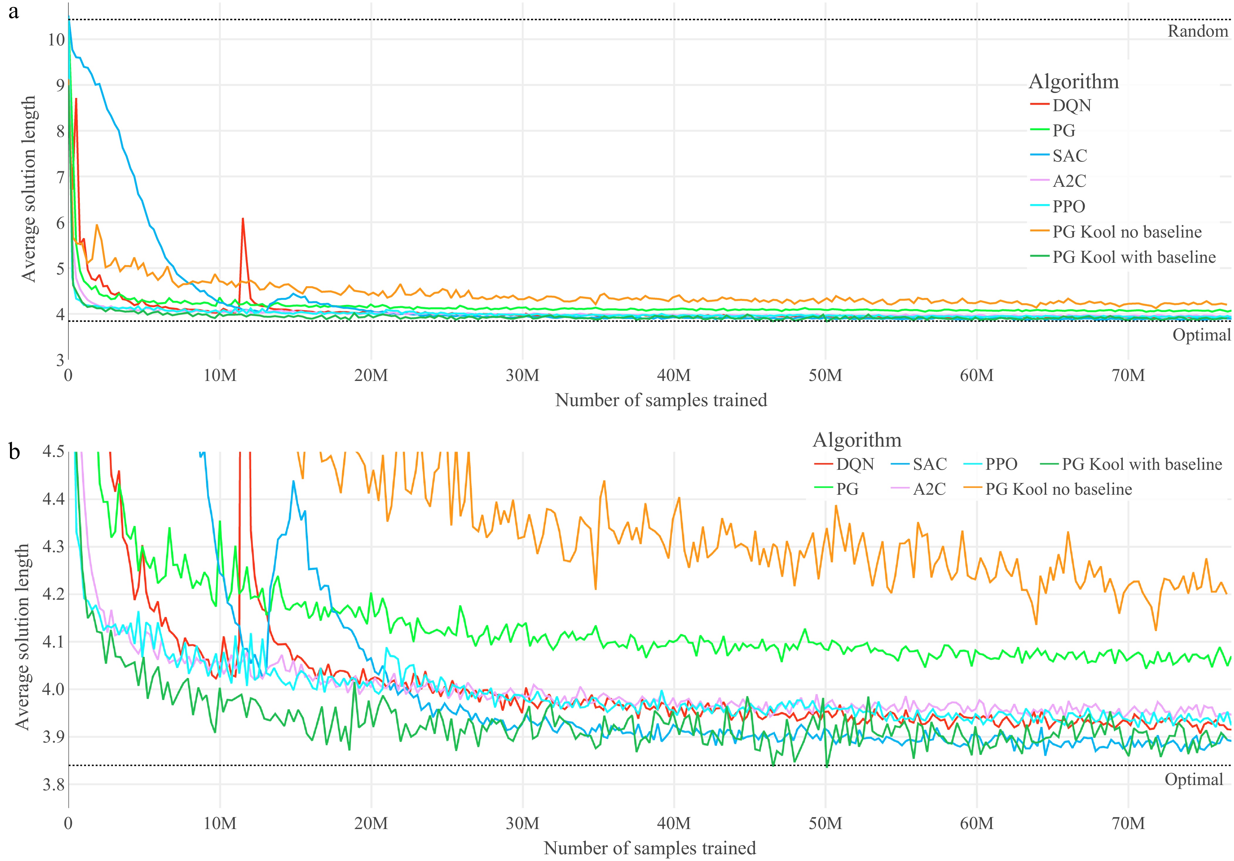
Figure 2. 

Training graphs of the optimized agents for the TSP. (a) Performance throughout the training of the seven optimized agents on TSP. (b) Magnified performance throughout the training of the seven optimized agents on TSP.

In these experiments, the PG algorithm without a baseline of Kool et al.^[45] performs worst and achieves a minimum average solution length of approximately 4.20. The main reason for this is likely the high variance in the gradient approximations, as Kool et al.^[27], use the vanilla PG calculation with full-trajectory realized rewards for reinforcing actions. This is the highest-variance variant because no baselines are used, and actions are reinforced based on previous steps in the trajectory. One way to reduce this variance in the gradient estimations, is by implementing the reward-to-go PG variant, as is done in Tianshou. In the experiments, this reward-to-go PG implementation of Tianshou outperforms the vanilla PG variant of Kool et al.^[27]. It reaches average solution lengths of approximately 4.08, while showing much more stable performance developments. Still, this PG variant is outperformed by algorithms like A2C and PPO.

The optimized A2C and PPO agents achieve peak performance values of approximately 3.94. As a reminder, A2C and PPO can also be considered PG algorithms with an advanced gradient formula. Instead of using Monte Carlo estimates of the expected value of a state-action pair, A2C and PPO implement Generalized Advantage Estimation, which can reduce the variance of the PG approximations. In these experiments, this variance reduction seems to occur, as A2C and PPO achieve significantly better results than the Monte Carlo PG variants without baselines. The bias introduced by the advantage estimates does not appear to be pivotal. In this final comparison, both A2C and PPO are characterized by high stability throughout the training. The additional objective function clipping of PPO has no significant effect in these final graphs, but reduced hyperparameter sensitivity, as outlined in Supplementary File 1 (Part 2.5).

The DQN implementation achieves a similar peak performance average of approximately 3.93. The fast convergence of this algorithm is likely possible through the short trajectory lengths and the addition of the second neural network for Double Deep Q-Learning, which reduces the overestimation bias at the start of training. At the 12 million sample mark, the agent suffers a momentary, drastic performance loss, which it recovers from in approximately one million additional training samples. Performance drops like this can be caused by the deterministic policies implied by the DQN algorithm, as tiny changes in the action values can cause drastically different decision trajectories by the agent.

The similar performances of DQN, A2C, and PPO demonstrate that PG methods are not always superior to value-learning. PG algorithms can not show their advantages in learning continuous actions for approximating solutions to TSP, as all actions are discrete. Furthermore, there is no necessity for stochastic policies when approaching TSP because there are no ambiguous observations of the environment.

The best training results of these experiments are achieved by SAC and the PG implementation by Kool et al.^[27] with their rollout baseline. These algorithms reach an average solution length of approximately 3.87 in this short training time. The SAC agent uses entropy temperature learning, which is why it improves slightly slower than the other algorithms at the beginning of training.

SAC learns Q-values of the current policy in an off-policy way. This variant of Q-value learning likely suffers less from overestimation bias than regular DQN, as no maximization operation is used. Possibly remaining overestimation bias is reduced in SAC by using two Q-value estimators, similar to Double DQN. Both of these details are likely the basis for the algorithm's fast learning and high performance. Additionally, exploration by entropy regularization might be another foundation of the algorithm's success, as in TSP, the actual values of some actions can be very close. With other exploration strategies, too much attention can be put on the maximum Q-value. Entropy regularization prevents the algorithm from committing too early to a promising strategy. Figure 3 displays some exemplary solutions of this best-performing (SAC) agent on TSP.

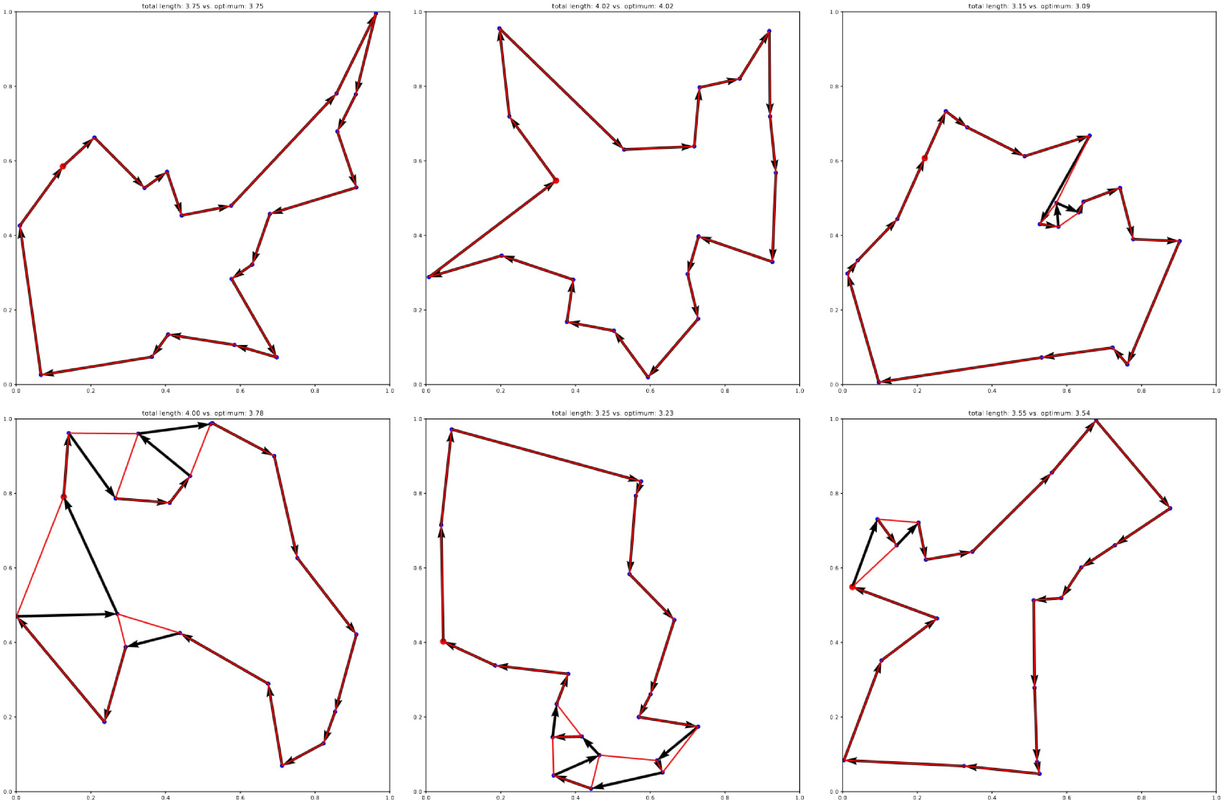
Figure 3. 

Exemplary solutions of the best-performing agent (SAC) on the 20-node TSP. Optimal solutions obtained with Gurobi are overlaid in red.

The second very successful algorithm in these experiments is the PG implementation by Kool et al.^[27] with the rollout baseline. The foundation of the success of this method must be the rollout baseline, as this is the only difference between this algorithm and the other worst-performing PG variant.

The vanilla PG estimation using the full-trajectory Monte Carlo returns is characterized by high variance. By subtracting the rollout baseline from the Monte Carlo returns, this variance seems to be reduced significantly when trained on TSP. One reason for this reduced variance is that the reinforcing term, i.e., the difference between the Monte Carlo returns with the rollout baseline, has an expected mean close to zero, and a low variance. This is the case because the trajectories taken by the trained policy and the rollout policy are very similar. Therefore, the state-values cancel out in expectation, and what remains are the full-trajectory advantage-values. Each action is reinforced by these full-trajectory advantage-values, which introduce some variance to the gradient estimations. This variance is dependent on the length of the trajectories, and those are relatively short for TSP with a problem size of 20. This factor and the other benefits presented likely make the vanilla PG variant with the rollout baseline so successful on TSP. The relatively high instability in the training graphs is likely caused by the relatively high learning rates and the divergence of the trained policy and the rollout policy in-between rollout updates.

Remark 1: Within the PG family, algorithms perform according to their gradient estimation variance. The vanilla PG variant has the highest variance and worst performance, followed by the reward-to-go PG implementation and the GAE PG methods (A2C, PPO). The vanilla PG algorithm by Kool et al.^[27] with their rollout baselines achieves the best results among the PG methods. This is likely because of the short trajectories in TSP and OP, and the fact that the rollout network explains a lot of the variance of the realized trajectory returns. The value-learners in DQN and SAC demonstrate some of the best results among all presented algorithms. They likely benefit from fast value propagation due to the short trajectories in TSP, and the bias reduction by their double critic architectures.

3.3.   Performance comparison for the orienteering problem (OP)

To further compare the performance of the algorithms, all of the agents are also trained on the OP. The results of these experiments are shown in Fig. 4.

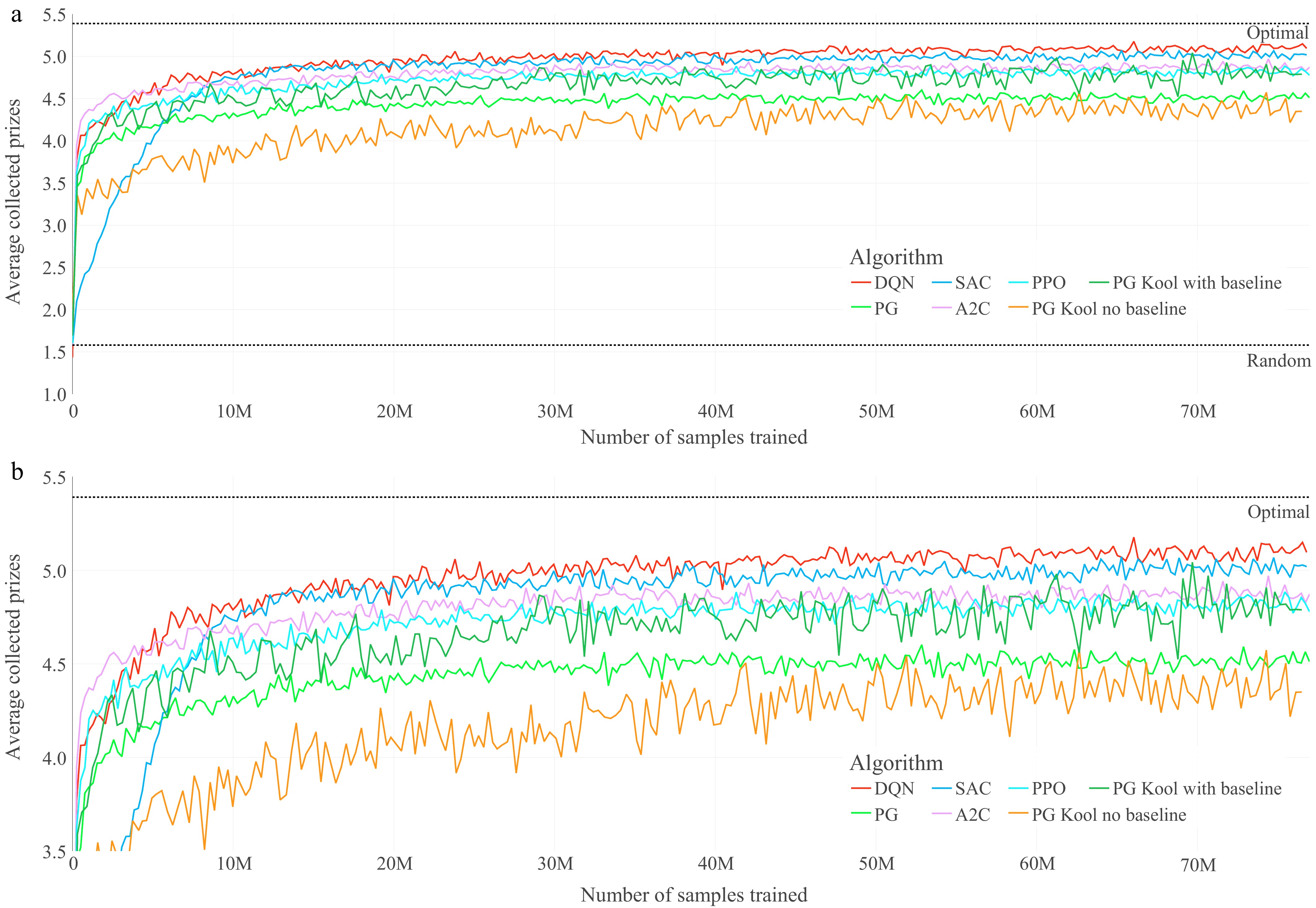
Figure 4. 

Training graphs of the optimized agents for the OP. (a) Performance throughout the training of the seven optimized agents on the OP. (b) Magnified performance throughout the training of the seven optimized agents on OP

As opposed to TSP, where the goal is to minimize the length of Hamiltonian cycles, in OP, the objective is to maximize the reward collected from different nodes with a limited tour length. All of the algorithms show continuous performance increments throughout the training and achieve significantly better results than a random policy (for the 20-node OP, 1.58 is the mean random performance, and 5.39 is the mean optimal performance^[27]). For reference, the performance specified by Kool et al.^[27] for their PG with rollout baseline on the 20-nodes OP is 5.19. This reference performance was achieved after significantly longer training than covered by the presented training graphs, and by selectively choosing the model of the best-performing training epoch. Similar to the results on TSP, the vanilla PG implementation without a baseline by Kool et al.^[27], performs worst in this setting as well, followed by the reward-to-go PG algorithm with a peak average score of ≈ 4.55. The A2C and PPO algorithms have similar training graphs and provide approximately the 3^rd and 4^th best results, with a peak average score of ≈ 4.85.

The main differences in the training results on TSP are established by the remaining three algorithms: DQN, SAC, and PG with the rollout baseline. In these experiments on OP, the PG algorithm with rollout baseline by Kool et al.^[27], only performs similarly well as A2C and PPO. It is quite significantly outperformed by the two value learners, DQN and SAC. Notably, although one of the most fundamental algorithms in this comparison, DQN achieves the best results on this test with a peak average performance of ≈5.10, followed by SAC with a corresponding value of approximately 5.02. One possible explanation for the lower relative performance of the PG method with rollout is that in the OP, the learned policy and the rollout policy can diverge faster, i.e., within fewer updates. This is because, in OP, not only the order of visited nodes can differ, but also the number and set of nodes visited. These possibly faster diverging models could lead to periodically larger variance in the advantage term and, therefore, larger periodic variance in the gradient estimations.

Remark 2: Most of the explanations presented in the TSP experiments can also be transferred to the OP training results. For example, the two PG algorithms without baselines are also performing worst in this setting because of their high gradient approximation variance. The two value-learner methods probably benefit from the even shorter trajectories of OP, and the disadvantages of $ \epsilon $-greedy exploration are probably also less pronounced due to the smaller state space than TSP. The PG variant with rollout baseline is not quite as successful on OP as on TSP compared to the other algorithms. One reason could be the faster diverging rollout and training policies, leading to periodically larger variance in the gradient estimations, depending on the rollout update frequency.

The choice of a transformer architecture for the models presented in this paper allows algorithms to be trained on different problem sizes without adjusting the neural networks, as they can handle variable input sizes and output sizes. Because of this, the models trained and evaluated on the 20-node TSP and 20-node OP can be used to approximate solutions to x-node instances. This section compares the generalization ability of the trained algorithms w.r.t. the problem sizes. For this comparison, TSP instances of 5, 10, 20, 30, 40, 50, and 100 nodes, and OP instances of sizes 20, 30, 40, 50, and 100 are examined. The corresponding plots are available in Figs 5 and 6, including random policies for comparison.

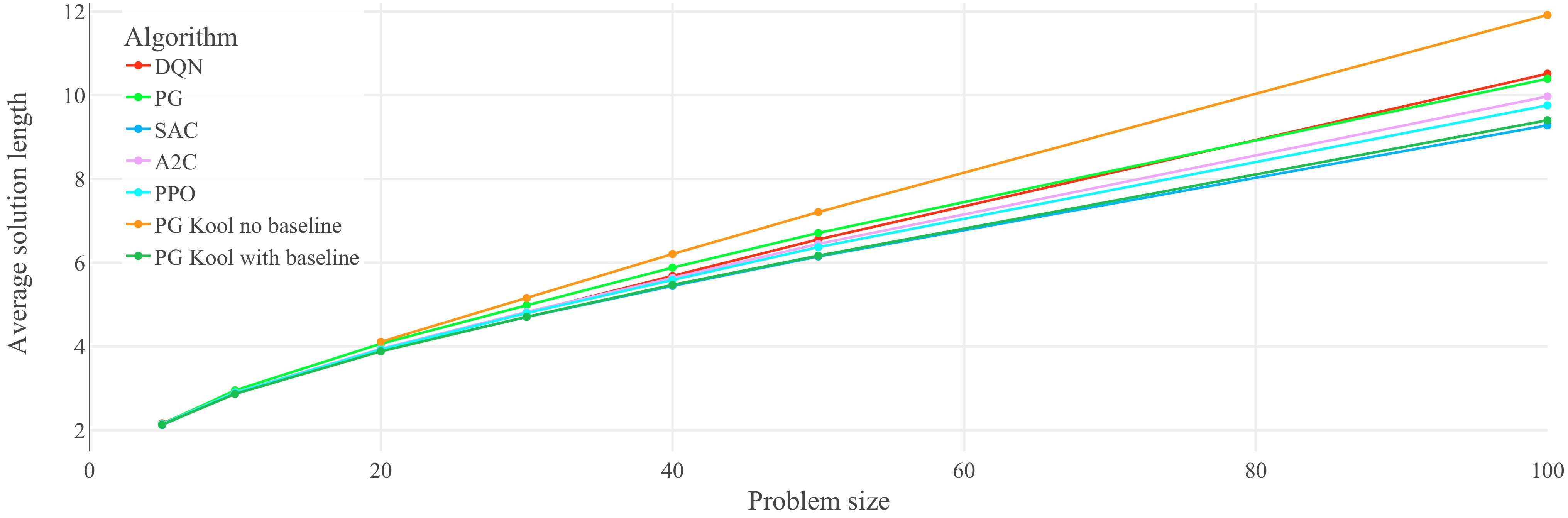
Figure 5. 

Performance on untrained problem sizes of the seven optimized agents on the TSP: generalization results for the TSP (lower is better). Each data point represents the average solution length of 1,000 evaluation problem instances. Lines between data points do not represent actual performance but are included for easier identification of trends. Refer to Table 1 for optimal and random solution lengths. The corresponding lines are not included in the plot in order to show the agents' performances on narrower axis scale.

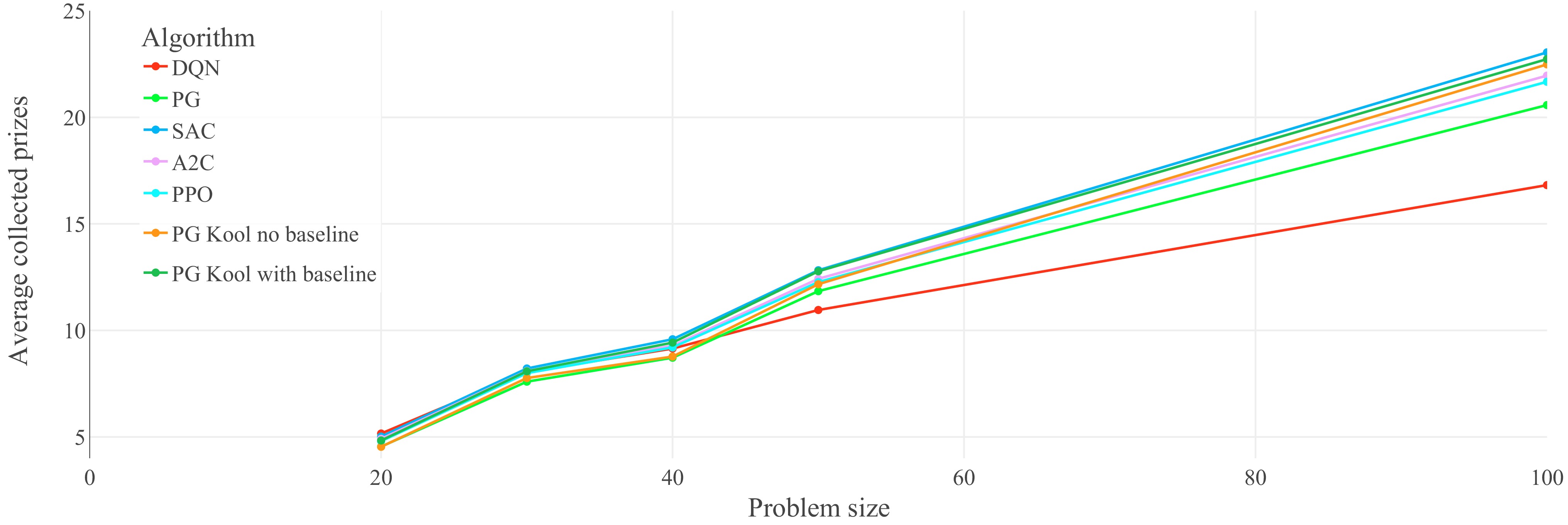
Figure 6. 

Performance on untrained problem sizes of the seven optimized agents on the OP: generalization results on the OP (higher is better). Each data point represents the average collected prizes of 1,000 evaluation problem instances. Lines between data points do not represent actual performance but are included for easier identification of trends.

One factor that can affect the generalization to unseen problem sizes is the type of policy learned, i.e., whether the policy is directly inferred from a value-estimator or whether a policy network defines the policy. Q-values, for example, are largely dependent on the problem size of the TSP and the OP. The chances of a value-estimator learning a valid function for many problem sizes are unlikely, especially if it is trained on instances of only one specific size. On the other hand, policy networks are not required to learn exact state-action values and have the ability to instead learn a general strategy or 'intuition' of which nodes to visit next.

The described disadvantage of value-based solutions for problem size generalization can be observed in Figs 5 and 6. While the DQN agent can compete with algorithms like A2C and PPO after training and evaluation on 20-node TSP, it becomes the worst-performing algorithm besides the PG of Kool et al.^[27], without baseline when evaluated on 100-node TSP (Fig. 5). This effect is even more pronounced for the OP in Fig. 6, where DQN suffers significant performance losses relative to the other algorithms. Notably, SAC also uses Q-value estimators during training, but they are only used to train a policy network based on the distributions implied by the Q-values. No Q-values are explicitly calculated at evaluation time, and the policy network solely defines the policy. For this reason, SAC does not suffer as much as DQN when evaluated on untrained problem sizes.

The ability of algorithms to generalize to unseen problem instances is very closely related to their robustness. Robustness describes the ability of an agent to handle changes in the environments between training and evaluation. One method that can improve the robustness of an algorithm is the use of maximum entropy RL, which lets the agent learn to handle disturbances during training. SAC is such a maximum entropy algorithm, and in the experiments of this paper, it shows the best generalization capabilities among the tested methods. In both Figs 5 and 6, the SAC agent has the best average performance on instances of size 100. Exemplary solutions of this SAC agent on the 50-node TSP are visualized in Fig. 7. The order of all the other algorithms largely remains unchanged when tested on unseen problem sizes.

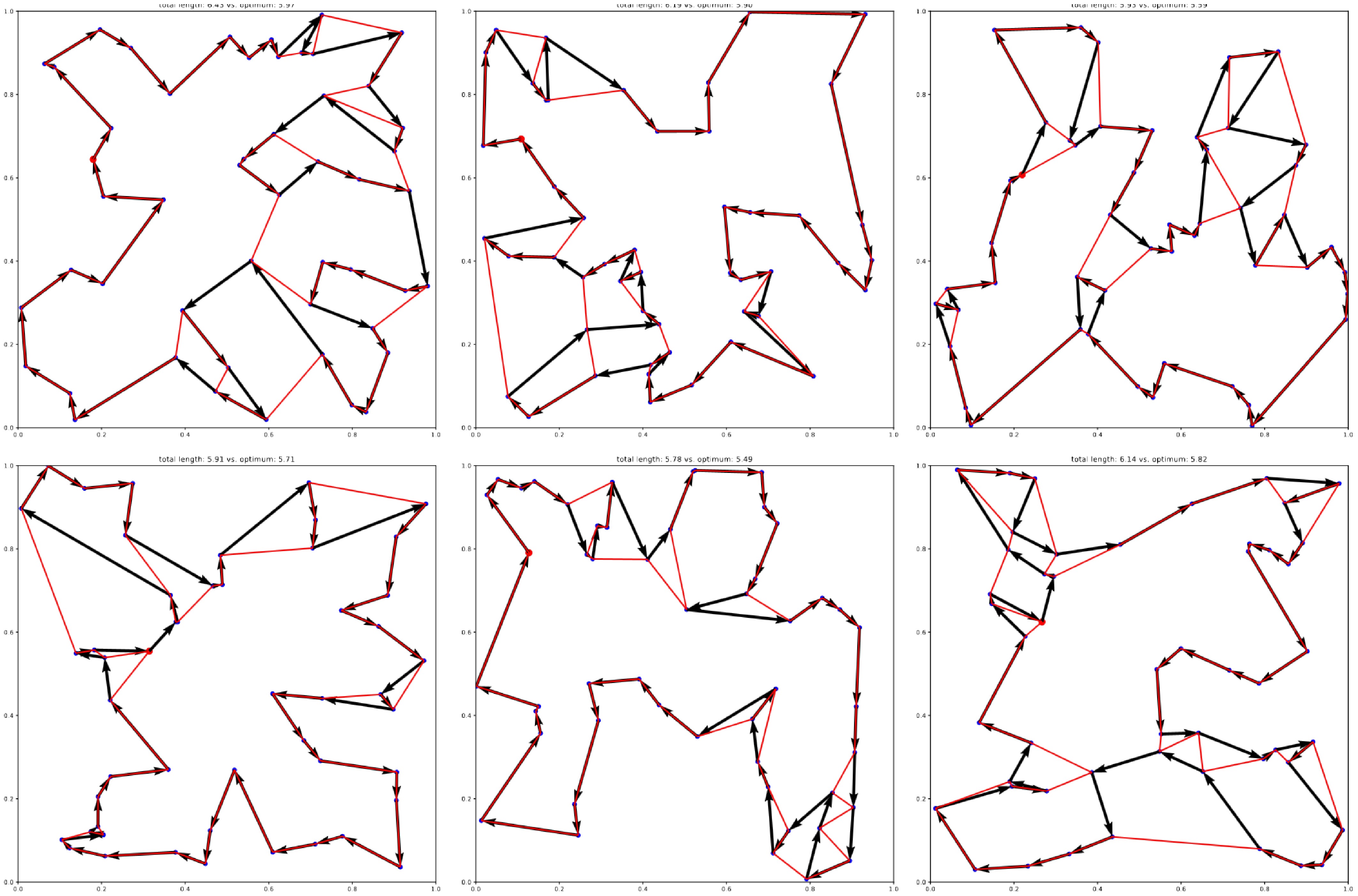
Figure 7. 

Exemplary generalization results of the best-performing agent (SAC) trained on the 20-node TSP, and evaluated on 50-node TSP instances. Optimal solutions obtained with Gurobi are overlaid in red.

Another strategy that can improve the robustness of an RL algorithm is to train it on a set of training environments that generate problem instances of different sizes. To test that theory, five of the agents from Fig. 5 were trained once again. This time, instead of only showing them 20-node problems during training, they were faced with one half of 15-node problems and another half of 25-node problems. This way, all of the compared agents have seen problems of the same size on average (i.e., 20). Finally, we used the respective trained agents and evaluated their average performance for TSP problems of different sizes, i.e., n = 20, 50, and 100.

Figure 8 and Table 2 show the results of the present experiments, which indicate that most agents trained on multiple problem sizes generalize better. Interestingly, some of the multi-problem-training agents even outperform their counterparts on problems of size 20, but the differences are mostly negligible. The trend towards larger untrained problems shows increasing generalization advantages of the multi-problem-training agents.

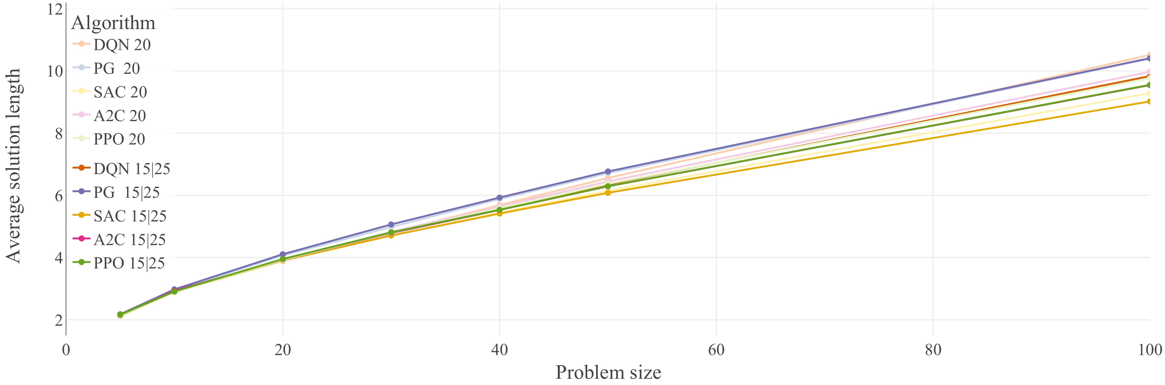
Figure 8. 

Performance comparison of five of the optimized agents from Fig. 5 (20-node problems), against the exact same agents trained on 15-node, and 25-node problems. Agents trained on 20-node problems have been assigned the lighter colors, while the agents trained on multiple problem sizes were assigned darker versions of the same colors. Generalization results for the TSP (lower is better). Each data point represents the average solution length of 1,000 evaluation problem instances. Lines between data points do not represent actual performance but are included for easier identification of trends

The main evaluation results are summarised in the following two remarks.

Remark 3: In the present experiments, drastic relative performance losses of the DQN agent were observed because its policy is defined by its value-estimations, and the state-action values in larger problem instances differ significantly from smaller ones. The ability of algorithms to generalize to larger problem instances is related to their robustness. SAC likely shows the best generalization capabilities through its robustness by maximum entropy exploration. The other algorithms, which do not include value-learning or additional robustness features, show a mostly unchanged relative performance for generalization.

Remark 4: The trained agent requires ≈22 ms per instance of size 50, and ≈45 ms per instance of size 100. Notably, the best-performing (SAC) agent on TSP outperforms the Gurobi^[2] optimal solver in execution time by a factor of 10, with problems of size 50 and by a factor of 20 with problems of size 100 (after overcoming the additional cost in training time), despite not being optimized for execution time as discussed. Still, the average optimality gap for 50-node instances is only ≈9%, and ≈19% for 100-node instances. Longer training of the agent, additional measures to improve the robustness, and execution time optimization can amplify the time benefits and improve optimality.

Moreover, the pretrained RL solutions, e.g., the SAC agent, remains applicable for large problem instances where solver-based or exact solution approaches are infeasible. The trained SAC agent requires ≈2 s per instance of size 1,000, and ≈25 s per instance of size 10,000.

The main results can be summarized as follows, cf. Remarks 1−4:

● The generalizing RL solutions of vanilla PG by Kool et al.^[27], as well as DQN and SAC perform well on the TSP and the OP for smaller problems (with e.g., 20 nodes).

● In the present experiments, SAC shows the best generalization capabilities for larger problems while being trained on smaller problem instances.

● Compared to optimal solutions, it is obtained that, e.g., a trained SAC agent computes TSP solutions of size 100 about 20× faster, while providing a decent optimality gap of below 20%.

● In contrast to optimal solutions, a trained SAC agent remains directly applicable to larger problems. For instances with, e.g., 1,000 nodes, the runtime is about 2 s.

● Further, it was found that agents trained on varied problem sizes tend to generalize significantly better.

5.2.   Limitations, potential extensions, and future work

This paper compares and evaluates the performance of selected RL algorithms for approximating solutions to combinatorial optimization problems. However, this work does not mark the end of research in this direction. Future work could expand on the range of algorithms selected in this paper, implement more exhaustive hyperparameter optimization solutions, and conduct detailed property-specific analysis. By comparing a wider range of algorithms, the bias-variance tradeoff could be analyzed in detail between all intermediate variants of the PG family or between DQN variants with other extensions like Dueling DQN.

An additional option that could improve the robustness of each algorithm would be an adversarial setup as proposed by Pinto et al.^[56], where an adversary tries to manipulate the problem sizes to values that the agent performs worst on. Further, the sensitivity of individual hyperparameters could be quantified more specifically by conducting more extensive experiments, as in the study by Liessner et al.^[57], for example. Furthermore, algorithms that generalize well to larger problem instances are desirable for RL on TSP and OP. This is because training on large problem instances would be much more time-consuming than training on small problems and applying the model to larger instances. Therefore, future work could conduct additional experiments for increasing the robustness of RL algorithms by implementing ideas like training on multiple problem sizes or developing an adversarial setup.

In this work, we selected, optimized, compared, and reasoned about state-of-the-art RL algorithms on the combinatorial optimization problems of the Traveling Salesman Problem and the Orienteering Problem. Out of the suitable options, DQN, PG, SAC, A2C, and PPO were selected to be optimized and compared against the variants by Kool et al.^[27]. Finally, the performance of optimized RL agents on the TSP and OP were compared, including experiments studying the algorithms' capability to be able to provide out-of-the-box solutions for generalized problem instances. Overall, the present results verified the high potential of RL algorithms applied to combinatorial optimization problems. Further, after all the experiments, the discrete version of SAC could be identified as the most effective RL algorithm for the TSP and OP. In future work, the results obtained could be extended to make selecting, optimizing, comparing, and reasoning on RL techniques applicable for a broader range of combinatorial optimization problems.