Rayleigh Generated Weibull distribution: properties and performance analysis

The development of modern statistical distributional models often involves integrating additional structural parameters into baseline distributions to enhance their empirical robustness. The Weibull distribution is one of the most widely used models in reliability analysis, survival studies, and engineering applications due to its mathematical tractability and ability to represent increasing or decreasing failure rates. However, real-world problems often exhibit more complex patterns that the classical Weibull model cannot adequately capture. In particular, empirical data sets often exhibit non-monotonic hazard behavior across varying tail characteristics, which motivates the development of more flexible generalizations capable of accommodating diverse distributional shapes. To address these limitations, several families of generalized distributions have been proposed by introducing additional parameters through generator mechanisms. One such approach is the Rayleigh Generated (RG) family of distributions, which has been shown to enhance modeling flexibility while preserving analytical tractability. Motivated by these advantages, this study introduces a methodology for formulating a three-parameter Rayleigh Generated Weibull (RGW) distribution by applying the RG mechanism introduced by Gaire & Gurung^[1] to the Weibull baseline model. The proposed RGW distribution possesses unique statistical properties and a more flexible hazard rate structure than the classical Weibull model and several existing extensions. In particular, the additional shape parameter introduced by the RG-family allows the model to capture complex failure-rate patterns and provides improved adaptability for modeling lifetimes and reliability data. Furthermore, the RGW distribution is investigated by deriving its statistical properties and estimating its parameters using the maximum likelihood method: simulation analysis and application to real datasets demonstrating its practical usefulness and modeling capability.

The remaining research work is organized as follows. In section 'Rayleigh Generated Weibull Distribution', a three-parameter RGW probability distribution is formulated, and some statistical properties and the rule for random number generation are derived. Section 'Method of parameter estimation using the method of maximum likelihood' presents the methods of parameter estimation, while section 'Numerical application' illustrates the numerical application and validation of the model using two real datasets. Section 'Simulation study' presents the simulation study of the model, and the last section concludes the paper.

Researchers have proposed numerous new families of probability distributions using transformation and generator techniques to enhance modeling flexibility and better capture complex data behaviors. Several generator-based distribution families have been introduced in the literature, including the Transmutation-G family^[2], Exponentiated-G family^[3], Marshall-Olkin-G family^[4], Zografos-Balakrishnan-G family^[5], Beta-G family^[6], T-X-G family^[7], and Exponential Arctan-G^[8], among others. These generator mechanisms extend baseline distributions by introducing additional shape parameters, thereby providing greater flexibility in modeling real-world phenomena such as actuarial data^[9], age-specific fertility rates^[10], age at first marriage^[11], reliability engineering^[12], and other demographic datasets. These applications demonstrate the flexibility and usefulness of generator-based distributions in capturing diverse patterns in empirical data. Motivated by these developments, the RG-family of distributions is adopted in this study to construct a new sub-model, referred to as the RGW distributions. The cumulative distribution function (CDF) and corresponding probability density function (PDF) of the RG-family of distribution are given as follows:

where, the $ g(x) $ and the $ G(x) $ are the PDF and the CDF of the base distribution to be chosen. Here $ F\left(x,\theta \right) $ is a valid CDF since it satisfies the boundary conditions; the baseline CDF $ G(x) $ is defined in [0,1], as $ G(x)\rightarrow 0 $, $ F(x)\rightarrow 0 $ and $ G(x)\rightarrow 1 $, $ F(x)\rightarrow 1 $.

Here, a flexible and widely used two-parameter Weibull distribution is chosen as the base; detailed applications of this distribution in the real world can be found in^[13,14]. The two-parameter Weibull distribution has a PDF and a CDF given as:

where, $ \alpha \gt ~0 $ is the shape parameter, and $ \beta \gt ~0 $ is the scale parameter.

Due to the simplicity, flexibility, and practical usefulness in modeling lifetime data, the Weibull distribution has been widely adopted as a baseline distribution for developing various generalized and modified models. Consequently, numerous extensions of the Weibull distribution have been proposed in the literature^[15−28]. Among these, some of the models have gained prominence by introducing two or three additional shape parameters. While these generalizations offer remarkable flexibility; they frequently encounter the problem of over-parameterization, where the increased parameter space leads to computational instability, over-parameterization, and significant challenges in maximum likelihood estimation for small to moderate sample sizes. On the other end of the spectrum, three-parameter models provide better parsimony but may lack the structural depth required to capture the complex tail behavior and specific skewness found in real-world data. The RGW distribution is strategically positioned to bridge this gap in the existing literature. The RGW maintains a parsimonious three-parameter structure, introducing only a single additional shape parameter $ \theta $ through a Rayleigh Generated transformation. This configuration allows the model to emulate the high-level flexibility of four and five-parameter distributions—specifically in capturing unimodal and heavy-tailed characteristics—while retaining the analytical tractability of simpler models. By providing a closed-form cumulative distribution function and a stable numerical framework, the RGW offers a computationally efficient alternative for researchers seeking a balance between mathematical precision and model parsimony, where data may be limited. Further discussions on extensions of the Weibull distribution can be found in Mohammad & Gaire^[8]. Motivated by these developments, this study introduces the RGW distribution by applying the RG-family of distributions to the Weibull distribution.

Probability density function of RGW distribution

The RGW distribution is obtained by applying the generator mechanism of the RG-family of distribution proposed in^[1] to a baseline Weibull distribution. According to the RG generator defined in Eqs (1) and (2), a new class of distribution can be constructed by transforming the baseline distribution through the Rayleigh Generated mechanism. By substituting the CDF and PDF of the Weibull distribution into Eqs (1) and (2), the CDF and PDF of the RGW distributions are derived and expressed in Eqs (5) and (6), respectively.

Although the generator structure follows^[1], the resulting distribution exhibits distinct statistical properties and hazard-rate behavior when the Weibull distribution is used as the baseline. The CDF and PDF of the RGW distribution are legitimate probability distributions since they satisfy the following defining properties of a probability distribution.

i. The boundary conditions: As $ x\rightarrow 0 $, $ F(x)\rightarrow 0 $, and as $ x\rightarrow \infty $, $ F(x)\rightarrow 1 $. Therefore, the CDF of the RGW distribution satisfies the boundary conditions.

ii. The non-negativity of the PDF: The PDF of the RGW distribution defined in Eq. (6) has three non-negative parameters. Here, $ {\left(\dfrac{x}{\beta }\right)}^{\alpha -1}\geq 0 $, for $ x> 0 $; $ \exp \left(-{\left(\dfrac{x}{\beta }\right)}^{\alpha }\right) $ and $ \exp \left(-{2\left(\dfrac{x}{\beta }\right)}^{\alpha }\right) $ are positive and $ \left[\exp \left(-{\left(\dfrac{x}{\beta }\right)}^{\alpha }\right)-\exp \left(-2{\left(\dfrac{x}{\beta }\right)}^{\alpha }\right)\right]\geq 0 $. Since every component of $ f(x) $ is non-negative, it follows that $ f(x)\geq 0 $.

iii. Normalization condition:

Since $ f\left(x\right)=\dfrac{d}{dx}F(x) $, which implies $ \int\nolimits_{0}^{\infty }f\left(x\right)dx $= $ F\left(\infty \right)-F\left(0\right)=1 $.

iv. Monotonicity:

As $ f\left(x\right)=\dfrac{d}{dx}F(x)\geq 0 $, which proves that the CDF is a non-decreasing function.

The graphical illustrations of the PDF and CDF of the RGW distribution for different parameter values are presented in Figs 1 and 2, respectively.

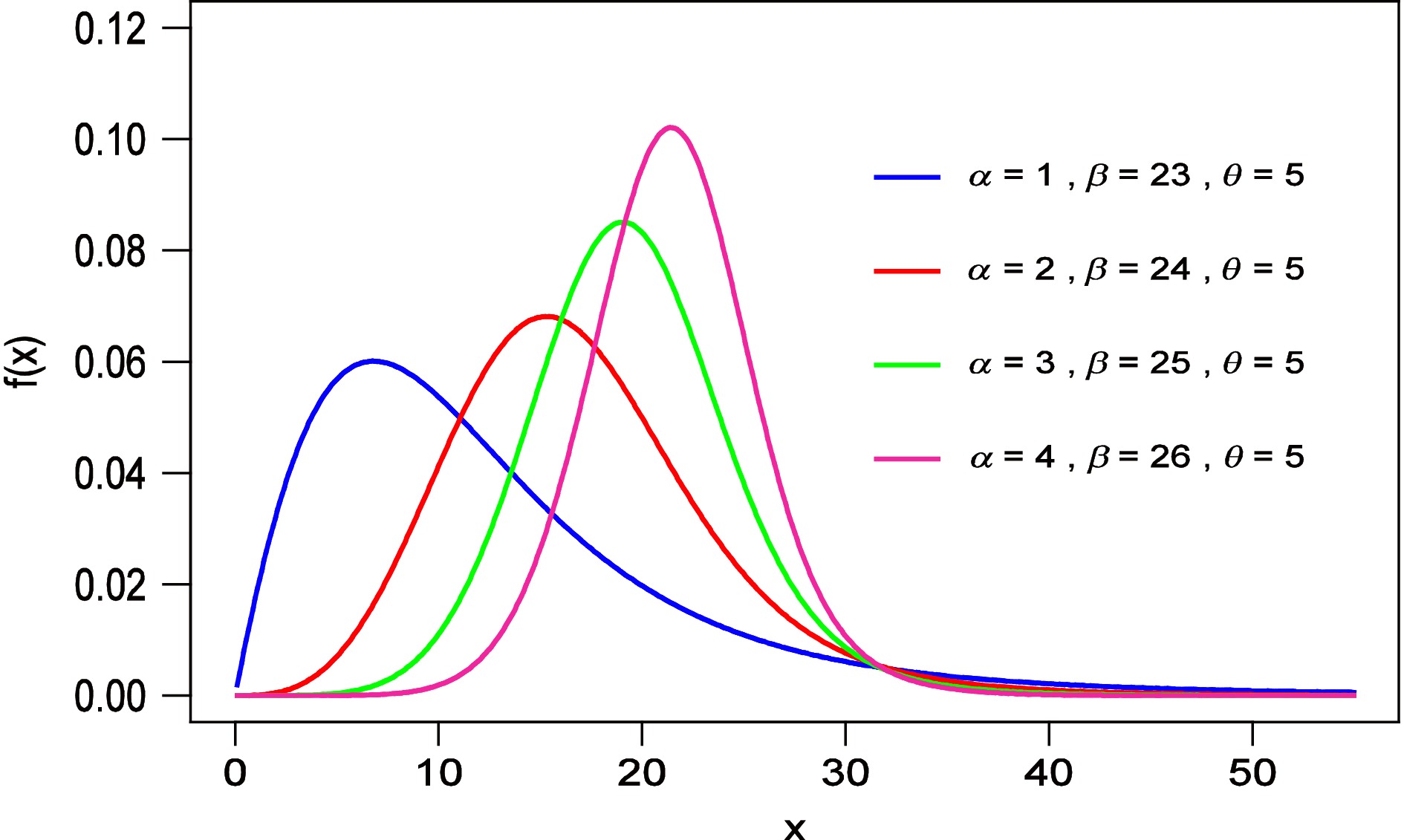
Figure 1. 

Graph of PDF of RGW distribution for different values of parameters.

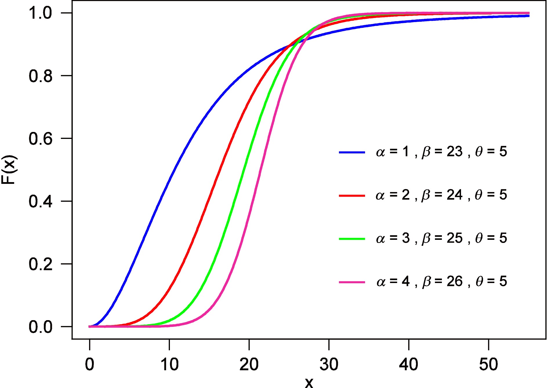
Figure 2. 

Graphs CDF of RGW distribution for different values of parameters.

Reliability analysis of RGW distribution

The probability that an event does not fail before time x is a reliability function. It is simply the complement of CDF (Rodrıguez^[29]), defined as $ R\left(x\right)=P\left(X> x\right)=~1-P\left(X\leq x\right)=1-F(x) $, where $ F(x) $ is the CDF of $ x $.

Thus, the reliability function of the three-parameter RGW distribution is given by Eq. (7), and its graphical representation is shown in Fig. 3 for selected parameter values.

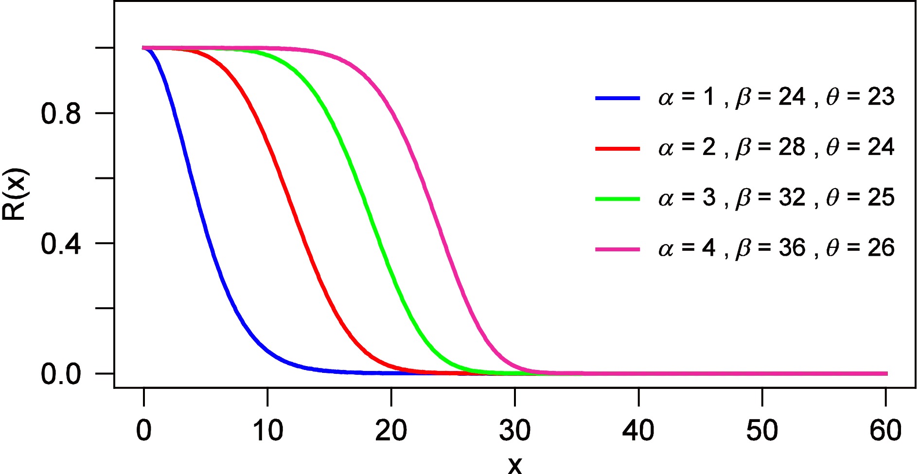
Figure 3. 

The reliability function of the RGW distribution.

Hazard, inverse hazard, and cumulative hazard rate function

The hazard rate function, which is the probability of failure of the random variable X, given that it has survived up to the time x, is defined as $ h(x)~=\dfrac{f(x)}{1-F(x)} $. Mathematically, the hazard rate function for the RGW distribution is well-defined based on Eq. (8). The hazard rate function is unique, increasing, and fluctuating after a certain point, and remains undefined beyond this point.

Figure 4 represents the hazard rate functions of the RGW distribution for selected parameter values. The curves exhibit diverse shapes, including nearly constant, increasing, and non-monotonic patterns. Notably, for some parameter combinations, the hazard fluctuates and terminates after a finite time, reflecting the model's ability to represent lifetime distributions with natural upper bounds. For the blue curve (α = 1, β = 23, θ = 5), the hazard rate remains nearly flat, suggesting an approximately constant failure rate, similar to exponential behavior. For the red curve (α = 2, β = 24, θ = 5), the hazard increases gradually after an initial low level, reflecting a monotonically increasing failure risk. For the green curve (α = 3, β = 25, θ = 5), the hazard starts small, rises moderately, then steepens, showing a non-monotonic pattern. Finally, for the pink curve (α = 4, β = 26, θ = 5): the hazard rises sharply after a delay, exhibiting a bathtub-like or late-accelerating hazard, often seen in biological survival data or in mechanical systems with wear-out phases.

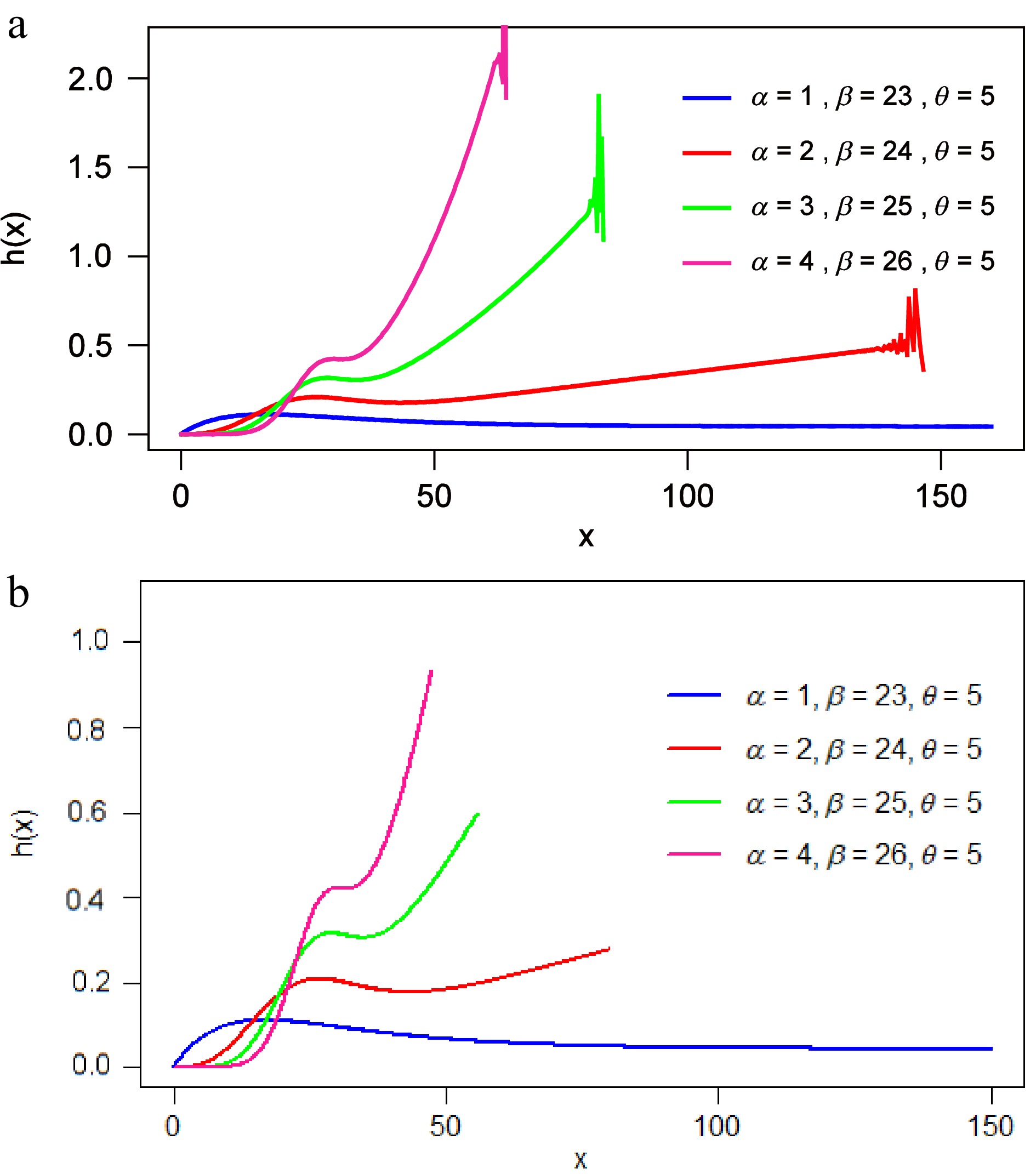
Figure 4. 

(a) Plot of the hazard rate function of the RGW distribution. (b) Clean plot of the hazard rate function of the RGW distribution.

Furthermore, the hazard-rate behavior of the RGW distribution demonstrates its flexibility compared to classical extensions of the Weibull model. As shown in Fig. 4, different parameter combinations allow the RGW to represent nearly constant hazards (resembling the exponential distribution), monotonically increasing hazards, and non-monotonic, bathtub-shaped hazards. This versatility is particularly valuable in survival and reliability analysis, where real-world systems often exhibit hazard functions that change direction over time. Unlike the classical Weibull, which is restricted to strictly increasing or decreasing hazard forms, the RGW can capture more realistic risk dynamics, thereby enhancing its practical applicability.

To rigorously evaluate the behavior of the hazard function $ h\left(x\right), $ as $ x\rightarrow \infty $, we examine the limit of Eq. (8). Let, $ {z=\left(\dfrac{x}{\beta }\right)}^{\alpha } $. As $ x\rightarrow \infty $, it follows that $ z\rightarrow \infty $ and $ \mathrm{exp} (-z)\rightarrow 0 $. The hazard function can be expressed as:

As x becomes large, we apply the Taylor expansion for the term $ {\left(1-\exp \left(-z\right)\right)}^{2}\approx $ $ \left(1-2\exp \left(-z\right)\right) $. Substituting this into the exponential term in the denominator:

Using the expansion $ \exp \left(1+\epsilon \right)\approx 1+\epsilon $ for small $ \epsilon $, the denominator becomes:

Substituting this back into the limit for $ h(x) $:

After canceling the common term, the expression simplifies to:

This mathematical derivation confirms that:

• For $ \alpha \gt 1 $, $ \underset{x\rightarrow \infty }{\lim } h\left(x\right)=\infty $, indicating a strictly increasing hazard, meaning the failure is more likely as time progresses; this is characterizing systems that undergo wear-out or aging, where the risk of failure increases over time.

• For $ \alpha =1 $, the hazard approaches a constant. This represents the memoryless property, where failure is independent of the system's age.

• For $ \alpha \lt 1 $, this represents a decreasing hazard rate, often seen in 'infant mortality' scenarios, where the probability of failure decreases as the entity survives the initial high-risk period.

These conditions prove that the fluctuations observed in Fig. 4a are computational iterations that were strictly numerical artifacts caused by the subtraction of nearly equal floating-point values in the denominator $ \left(-\theta {\left(1-\exp \left(-z\right)\right)}^{2}\right)-\mathrm{exp} (-\theta ) $ as they both converged to $ \mathrm{exp} (-\theta ) $. By identifying that the power-law term governs the limit $ {\left(\dfrac{x}{\beta }\right)}^{\alpha } $. It demonstrates that the model is mathematically stable and physically interpretable throughout its entire support.

In Fig. 4a, the hazard function appeared to fluctuate in the extreme right tail. A rigorous examination revealed that these fluctuations were not a theoretical property of the distribution, but were caused by catastrophic cancellation in the floating-point subtraction within the denominator. As x increases, the survival function approaches zero, and the computer is forced to calculate the difference between two values that are identical within machine precision approximately 10⁻¹⁶.

To ensure scientific accuracy, the visual representation in Fig. 4b has been adjusted. We improved the numerical stability of the computations by using Python's expm1 function and truncating the curves where the survival function falls below 10⁻⁷. Figure 4b now displays the corrected hazard rate functions. By removing the unstable terminal noise, the figure clearly demonstrates the smooth, monotonic increase in the hazard for $ \alpha \gt 1. $ These results confirm that the model is numerically stable and physically interpretable across the distribution's statistically significant support, successfully capturing the intended reliability characteristics without interference from computational artifacts.

Similarly, the reverse (or inverse) hazard rate function of a continuous distribution is defined as $ rh\left(x\right)=\dfrac{f\left(x\right)}{F\left(x\right)},x> 0 $. For the RGW distribution, substituting the expression of $ f(x) $ and $ F(x) $ given in Eqs (6) and (5) into this definition, and after simplification, the reverse hazard rate function is expressed in Eq. (9) as:

The cumulative hazard rate function of the RGW distribution is given by Eq. (10). Furthermore, Fig. 5 shows cumulative hazard rate functions for different parameter values.

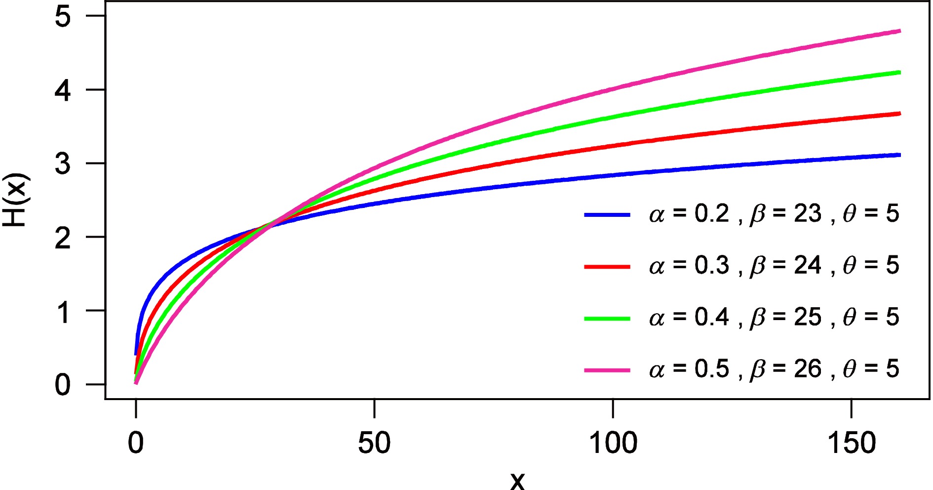
Figure 5. 

Plot of the cumulative hazard rate function of the RGW distribution.

Random number generation of the RGW distribution

To generate the set of random variables that follows the RGW distribution, a method of inversion from the CDF has been used; for this, assume $ F\left(x\right)=u $, where $ u $ is a function that follows the uniform distribution in [0, 1].

Further, simplification from this equation gives the value of the random variable $ X $ that follows the RGW distribution as derived,

Equation (11) can be used to generate the set of random variates $ X $ for the RGW distribution from the given value of parameters α, β and θ. Similarly, this equation also serves as the quantile function of the RGW distribution.

Let, $ {X}_{1},{X}_{2},\cdots ,{X}_{n} $ to be a random sample of size n from the RGW distribution, having a PDF defined in Eq. (5). The likelihood function of the RGW has been expressed as:

To determine the most likely parameter values, we operate on the logarithm of the likelihood function to get the Log-likelihood function, which is formulated as follows:

The likelihood function is obtained by multiplying the density of the independent observations. For computational convenience, the natural logarithm of the likelihood function is taken, converting the product into a sum and simplifying the derivation of the maximum likelihood estimators (MLEs). To estimate the MLE of parameters involved in the RGW distribution, the components of the score vectors can be generated by taking the first derivative of the $ \ln L $ with respect to the parameters as:

After equating these partial derivatives to zero, systems of nonlinear equations will be obtained. A simple calculation cannot produce the MLE for the unknown parameters of the GRW distribution. Suitable numerical nonlinear optimization algorithms, such as the Newton-Raphson method are needed to maximize the likelihood function.

Two real data sets were taken to test the proposed model's flexibility, suitability, and validity. We initially validate our model using a well-known 100-point sample representing bank customer service intervals, as documented by Ghitany et al.^[30], and also utilized by Gaire & Gurung^[31]. The second dataset comprises 128 data points on the remission times (in months) of bladder cancer patients. In this dataset, remission time is defined as the decrease or disappearance of cancer after treatment, as described by Lee & Wang^[32]. Goodness-of-fit and parameter estimates for the fitted distributions were obtained using the R programming language.

The validity tools applied to validate the model fitting are the negative log-likelihood (NLL), Akaike information criterion (AIC), Bayesian information criterion (BIC), Anderson-Darling (AD) test, and Cramér–von Mises (CVM) test. The OPTIM function available in the R programming language^[33] using the Adequacy Model^[34] has been used to estimate the parameter associated with the RGW distribution. The algorithm used to estimate the parameters were the Broyden–Fletcher–Goldfarb–Shanno (BFGS) method.

The RGW model was applied to fit two real-world data sets, and the parameters were estimated using MLE, the expression derived above in this study. The fitted results using an RGW distribution for both data sets are compared with those from a two-parameter Weibull distribution (Eq. [1]), a three-parameter transmuted Weibull (TrW) distribution (Eq. [17]), a four-parameter Kumaraswamy Weibull (KuW) distribution (Eq. [18]), a Beta Weibull (Beta-W) distribution^[18], and a Marshall-Olkin Weibull (MO-W) distribution^[4]. Estimated parameter values and test statistics for the waiting time data under the different models are presented in Table 1. Further, Fig. 6 presents histograms of the empirical and fitted values of customers' waiting time for different models.

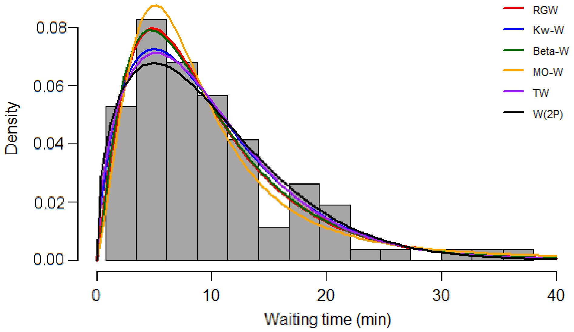
Figure 6. 

Histogram of observed and fitted lines of values of the number of customers for waiting time.

Figure 7 presents P-P plots of waiting-time data to assess the visual adequacy of the RGW model. All models provided a reasonable fit; the RGW model, the greed one, exhibited the closest adherence to the diagonal reference line, particularly in the median and upper quantile regions, as indicated by the different test result matrices.

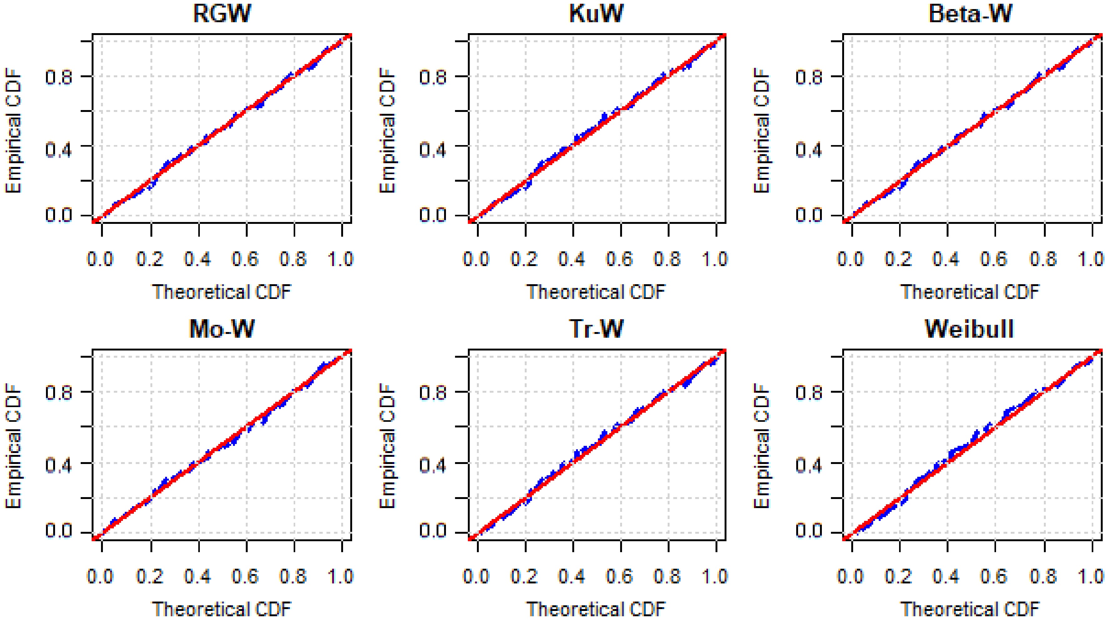
Figure 7. 

P-P plot of customers for waiting time.

Based on the goodness-of-fit results, the RGW distribution provides the best fit among the considered models for customers' waiting time. It has the lowest NLL (316.95), AIC (639.89), and BIC (647.70). The smallest values of NLL, AIC, BIC, AD, and CVM test values for the RGW distribution indicate superior model performance in balancing overall goodness of fit and parsimony among the comparative models. Additionally, the KS test results indicate that the RGW distribution yields the smallest KS statistic (0.0376), the highest p-value (0.9989), the lowest AD test value (0.127), and the lowest CVM test value (0.017). These KS results, which are in strong agreement with the RGW-fitted results, are in good agreement with the observed data. The AD test suggests that the RGW model captures the data's extremes better than the other models. Similarly, the CVM test result indicates that the overall distance between the fitted result and observed distribution is smallest for RGW. Thus, the RGW distribution is the most appropriate model for describing customer waiting times in this dataset among the compared models.

In the same manner, estimated parameter values and test results for different statistics on the remission time data are presented in Table 2. The histograms of the observed and fitted patient counts are shown in Fig. 8.

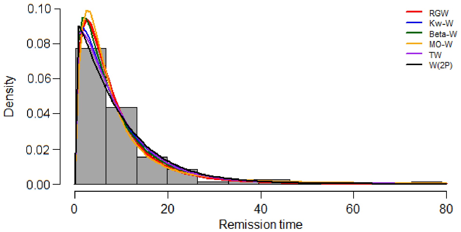
Figure 8. 

Empirical and fitted number of patients against remission time.

A similar analysis of remission time data indicates that the RGW distribution is the best-fitting distribution among those considered. It produces the lowest NLL (409.824), AIC (825.6489), and BIC (831.3846), indicating its superiority in balancing model complexity and goodness of fit, and providing the best model fit among the four distributions. Additionally, the KS, AD, and CVM test results confirm strong agreement with the observed data, as the RGW model has the lowest KS statistic (0.0344), the highest p-value (0.9981), the lowest AD (0.127), and the lowest CVM (0.017), indicating an excellent fit. The RGW distribution is the most appropriate model for accurately describing remission times among the selected distributions.

Figure 9 presents the P-P plots of remission times for patients with bladder cancer to provide a graphical qualitative assessment of the model. In this case, the RGW model exhibits the most consistent adherence to the diagonal reference line across all quantiles, demonstrating that it effectively captures the underlying distribution of remission times and further validating its superiority, as suggested by multiple validity test result matrices.

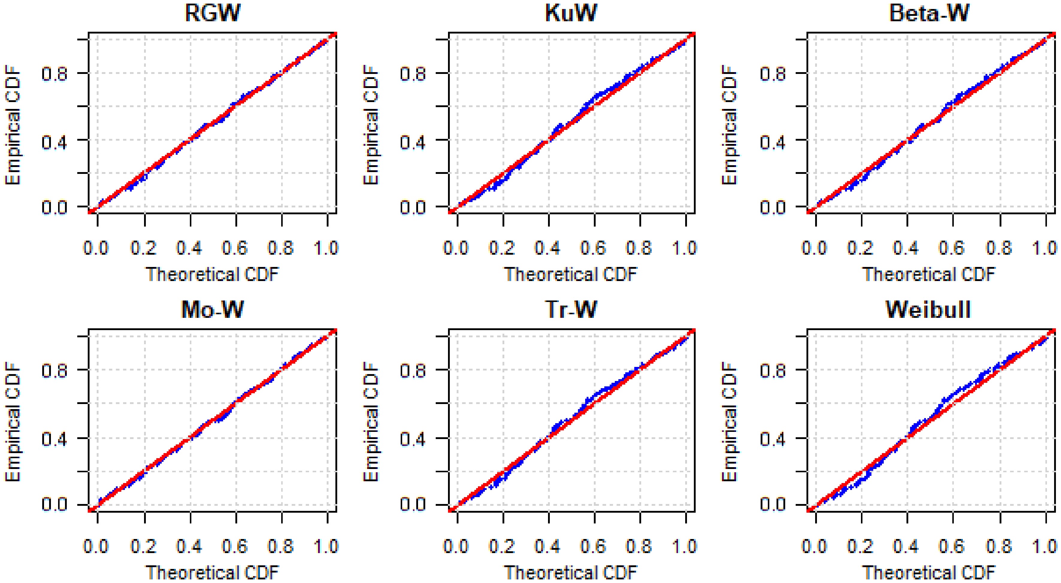
Figure 9. 

P-P plot of remission time.

The performance of the MLEs discussed in parameter estimation section for the RGW distribution was evaluated via a Monte Carlo simulation. Three distinct sets of true parameter values were tested across sample sizes n = 100, 200, and 500, with N = 1,000 iterations per sample size. The random numbers were generated using Eq. (11). The numerical results of the evaluation, Tables 3−5, were summarized and included the estimated mean, bias, and mean squared error (MSE).

The simulation study results for three sets of parameter values provide evidence of the asymptotic consistency of the MLEs for the RGW distribution. The initial observations indicate that the MSE consistently decreases as the sample size increases from 100 to 500 across almost all parameters. Such downward trends in MSE indicate that the estimators become more precise and converge toward the true parameter values as more data become available. In the presence of bias, the estimators exhibit a general trend of convergence toward zero as the sample size increases, though some parameters, such as theta in the third set, show persistent negative bias in smaller samples. The shape parameter alpha tended to show a slight overestimation across all sets, while the scale parameter beta remained relatively stable with low MSE. In general, as the sample size increases, both bias and MSE decrease, which supports the use of MLE to estimate the parameters of the RGW distribution.

Figures 10 and 11 present the visual comparisons of bias and MSE for the simulation results across the three parameter sets. The bias plot shows that the bias for each parameter changes with increasing sample size across the three sets. It is observed that most parameters converge toward the zero line as the sample size increases, suggesting that the estimators are asymptotically unbiased. Similarly, the MSE plots clearly show a downward slope for all parameter selections. As the sample size increases, the variation in parameter estimates decreases, indicating that the model is statistically consistent. For the third parameter, theta shows higher sensitivity, suggesting that for very large theta values, even a larger sample size might be required to achieve significant convergence.

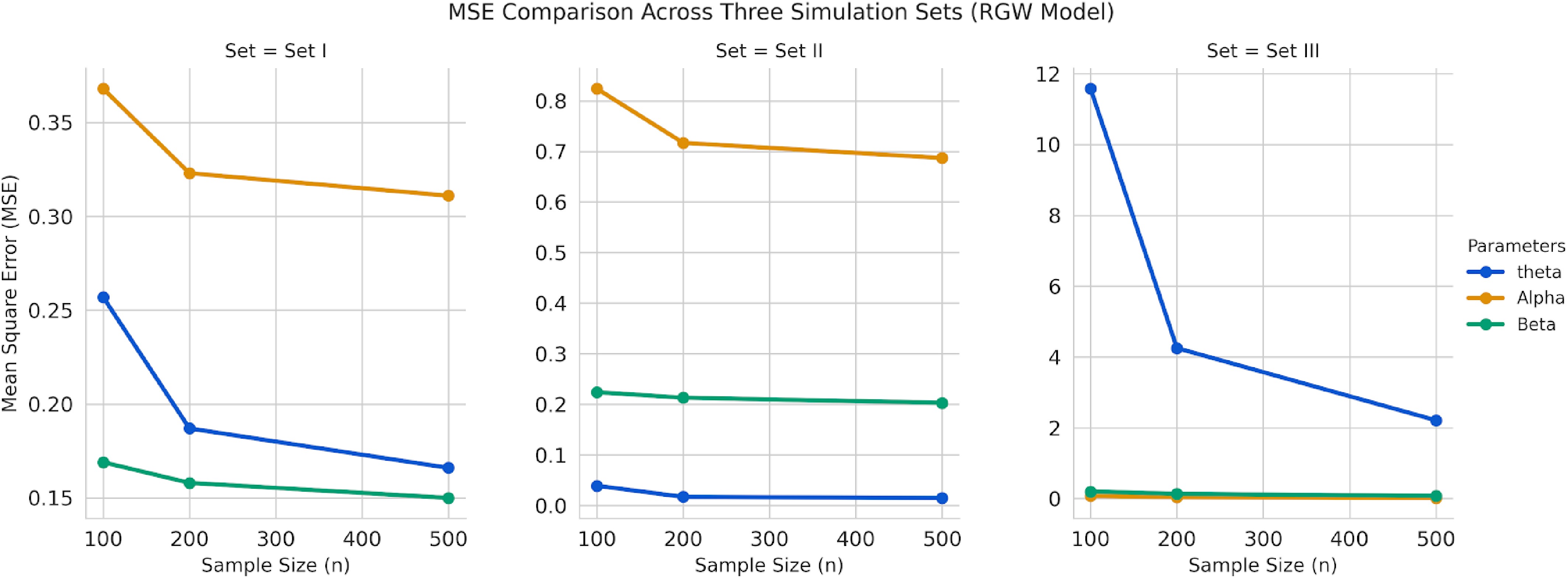
Figure 10. 

MSE comparison across parameter sets for RGW simulation.

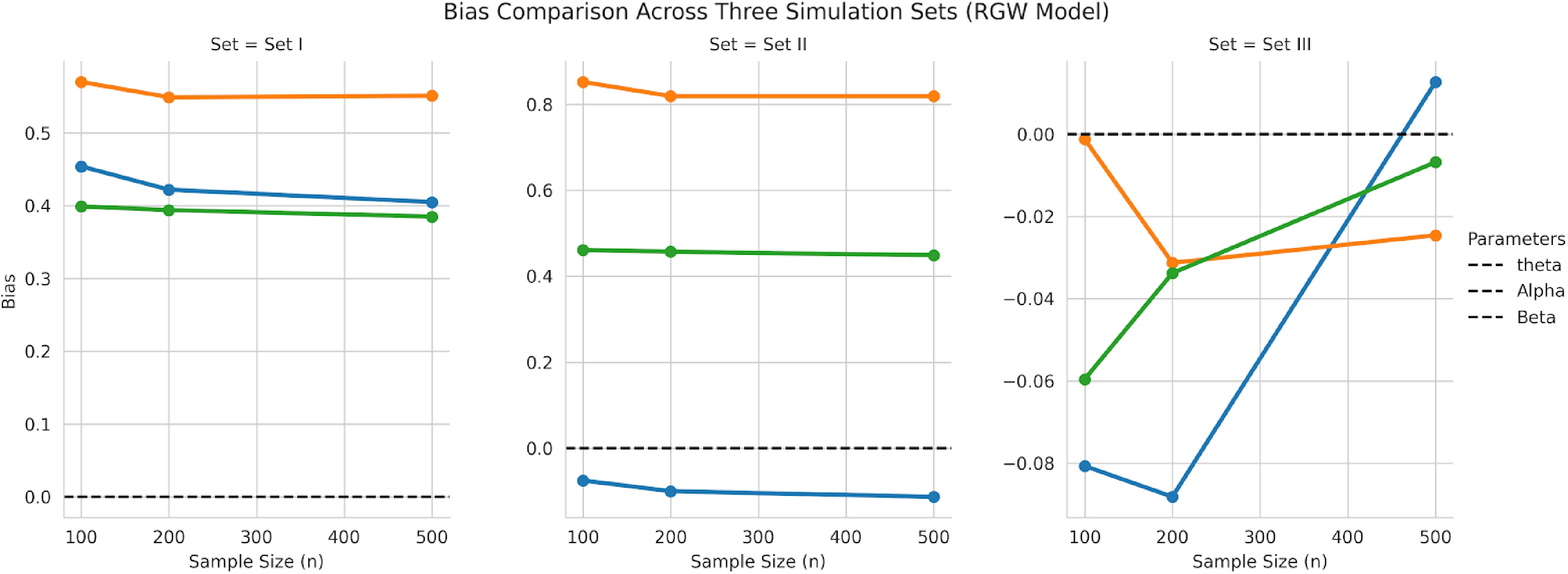
Figure 11. 

Bias comparison across parameter sets for RGW simulation.

The RGW distribution, a sub-model of the RG-family of distributions, has been presented. The relationships for estimating the parameter using the MLE and random number generation are derived, and certain statistical features of the distribution are examined. The hazard curves of this distribution exhibit a variety of forms, including non-monotonic, rising, and almost constant patterns. The simulation results verify that as the sample size increases, the MLE consistently yields estimates of the RGW distribution parameters that are progressively more accurate. To assess the performance of the RGW distribution, two datasets were employed: bank queue length, and patient remission intervals. As validity tools, a variety of test statistics have been employed, including AIC, BIC, KS, AD, and CVM. From the diverse validity test statistics and the P-P plot, it was found that the RGW model is sufficiently flexible to better fit the data than the other compared models.