


-
In the MCR-WPT system, the resonant frequency of the system is often a fixed value. The transmission efficiency or transmission power of the system reaches the maximum value at the resonant frequency, but due to various reasons in the actual operation process, such as the distance between the transmitting and receiving coils is too close, the coupling coefficient increases due to too many turns, and the mismatch of the load resistance value of the system, etc., the power will be output at two or more frequencies other than the original resonant frequency, resulting in frequency bifurcation[1,2].
In fixed-frequency systems, conventional SS compensation methods primarily involve compensating for self-inductance and mutual inductance[3]. While these methods can initially improve power transfer efficiency, they suffer from several limitations in dynamic operating conditions. For instance, in electric vehicle wireless charging scenarios, changes in coil alignment due to vehicle movement or road surface irregularities can lead to a shift in system parameters, reducing transmission efficiency, and causing voltage fluctuations[4,5]. Similarly, in mobile device wireless charging, variations in load resistance due to battery state-of-charge changes can significantly affect power stability, making it difficult to maintain optimal performance using traditional SS compensation techniques.
To address these challenges, SS series compensation topologies with primary-side detuning have been introduced in fixed-frequency systems. By carefully adjusting the detuning rate of the primary-side compensation network, these systems can accommodate a wider range of coupling coefficient variations, allowing for relatively stable power transfer in practical applications[6]. However, this approach still faces limitations when the coupling coefficient fluctuates significantly, as it cannot dynamically adjust the operating frequency to match optimal conditions.
On the other hand, frequency-adaptive SS topologies based on PT symmetry have demonstrated superior performance in frequency conversion systems[7−9]. Unlike fixed-frequency systems, these topologies leverage the system's state variables—such as inductor current and capacitor voltage—to achieve self-regulated operation without external intervention[10−12]. This enables them to maintain a nearly constant output voltage regardless of coupling coefficient variations or load changes, which is highly beneficial in practical scenarios[13,14].
Compared to traditional compensation methods, frequency-adaptive SS compensation not only improves transmission efficiency and system robustness but also simplifies circuit design by reducing the need for complex real-time control algorithms. Additionally, it lowers manufacturing and maintenance costs, making it particularly advantageous for large-scale deployment in applications such as electric vehicle charging infrastructure, mobile electronics, and high-power industrial wireless power systems.
This paper systematically analyzes the specific operating frequency characteristics of the autonomous wireless power transmission system based on its frequency adaptation properties. Furthermore, it explores the advantages of frequency conversion systems over fixed-frequency systems, highlighting their potential to enhance efficiency, stability, and cost-effectiveness in real-world applications.
-
Figure 1 shows a typical series series compensation topology, where M represents the mutual inductance of the coil and L1 and L2 are the equivalent inductances of the transmit and receive coils, respectively. R1 and R2 are the equivalent resistances of the transmitting coil and the receiving coil, respectively. C1 and C2 are resonant capacitors at the transmitter and receiver. Zref is the reflected impedance reflected back to the transmitter at the receiving end, and Zin is the input impedance. RL is the equivalent load resistance. ω represents the operating angular frequency of the system, which has:
$ {Z_{{\text{ref}}}}(j\omega ) = \dfrac{{{{(\omega M)}^2}j\omega {C_2}}}{{({R_{\text{L}}} + {R_{\text{2}}} + j\omega {L_{\text{2}}})j\omega {C_{\text{2}}} + 1}} $ (1) $ {Z_{{\text{in}}}}(j\omega ) = \dfrac{1}{{j\omega {C_1}}} + j\omega {L_1} + {Z_{{\text{ref}}}} + {R_1} $ (2) 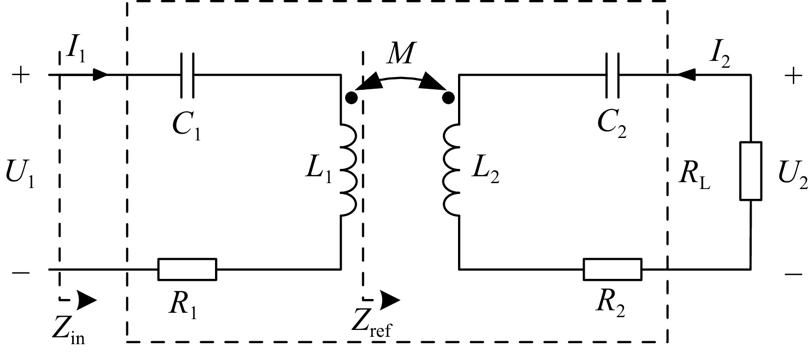
Figure 1.
Topology of S/S compensated WPT system.
When the system works in a fully resonant state, the phase angle of the input impedance is 0, that is, the imaginary part of Zin is 0, and the following results can be obtained:
$ a{\omega ^6} + b{\omega ^4} + c{\omega ^2} + d = 0 $ (3) where a, b, c, d is:
$ \left\{\begin{gathered}a=C_1C_2^2L_2\left(L_1L_2-M^2\right) \\ b={{-}}C_2^2L_2^2+C_1C_2\left(M^2+L_1\left(-2L_2+C_2\left(R_2+R_{\text{L}}\right)^2\right)\right) \\ c=C_1L_1+2C_2L_2-C_2^2\left(R_{\text{2}}+R_{\text{L}}\right)^2 \\ d=-1 \\ \end{gathered}\right. $ (4) Solving Eqn (3), we can find the three roots of ω, ω1, ω2, ω3, the corresponding frequencies are f1, f2, f3, if the compensation capacitance value is set so that the natural oscillation angle frequency ωp of the primary side is the same as the natural oscillation angle frequency ωs of the secondary side, then there are:
$ {\omega _{\text{p}}} = \dfrac{1}{{\sqrt {{L_1}{C_1}} }} = {\omega _{\text{s}}} = \dfrac{1}{{\sqrt {{L_2}{C_2}} }} $ (5) In this case, Eqn (3) can be reduced to solving the following two equations:
$ \left\{ \begin{gathered} 1 + \left( { - 2{C_1}{L_1} + {C_2}^2{{({R_{\text{L}}} + {R_2})}^2}} \right){\omega ^2} + \left( {{C_1}^2{L_1}^2 - \dfrac{{{C_2}^2{L_2}{M^2}}}{{{L_1}}}} \right){\omega ^4} = 0 \\ 1 - {C_1}{L_1}{\omega ^2} = 0 \\ \end{gathered} \right. $ (6) Let
$\Delta = \left\{ {\left( { - 2{C_1}{L_1} + {C_2}^2{{({R_{\text{L}}} + {R_2})}^2}} \right)} \right\} - 4\left( {{C_1}^2{L_1}^2 - \dfrac{{{C_2}^2{L_2}{M^2}}}{{{L_1}}}} \right)$ $ \left\{ \begin{array}{ll} {Z_{{\text{in}}}} = \dfrac{{{\omega ^2}{M^2}}}{{{R_{\text{L}}} + {R_2}}} + {R_1}&\omega = {\omega _2} \\ {Z_{{\text{in}}}} = \dfrac{{({R_{\text{L}}} + {R_2}){L_1}}}{{{L_2}}} + {R_1}&\omega = {\omega _1},{\omega _3} \end{array} \right. $ (7) Under the resonant frequency, the system is reflected in the negative resistance characteristics, at the f1 and f3 frequencies, the system input impedance is independent of the coupling coefficient, if the system can track the f1 and f3 frequencies, the system output is decoupled from the coupling coefficient, and has strong output robustness. The T-equivalent model and simplified model of the system at three frequencies of full resonance are shown in Fig. 2, the red dashed box represents the splitting of the compensation capacitor, while the black dashed box indicates the complete resonance of internal components. The diagram illustrates the three states of capacitor compensation under the three resonance frequencies of the system. In the next section, we will show how to implement frequency adaptation through hardware circuitry, so that the system can track one of the frequencies of the fully resonant frequency.
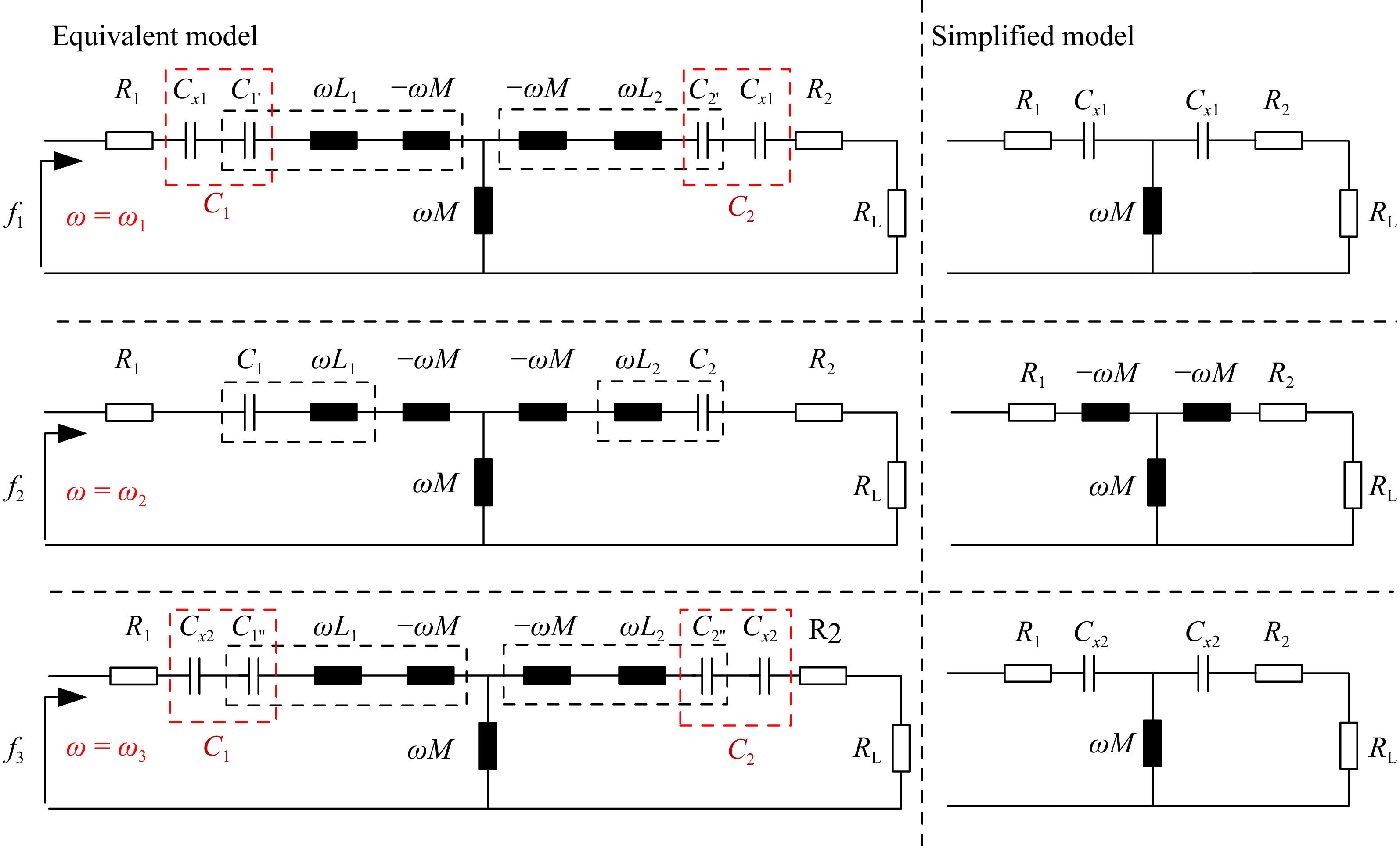
Figure 2.
T-equivalent model and the simplified model when Im(Zin) = 0.
-
As shown in Fig. 3, the system adopts a full-bridge high-frequency inverter circuit as the power output circuit, and achieves frequency adaptation through the control structure shown in Fig. 4.
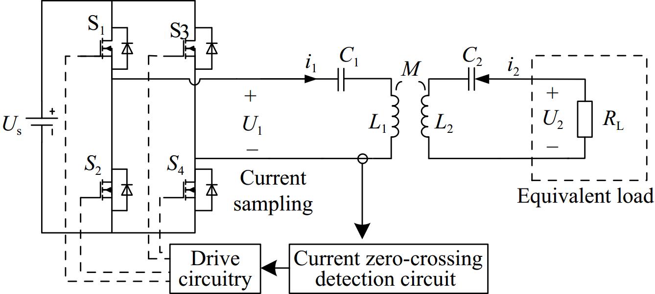
Figure 3.
Circuit implementation.
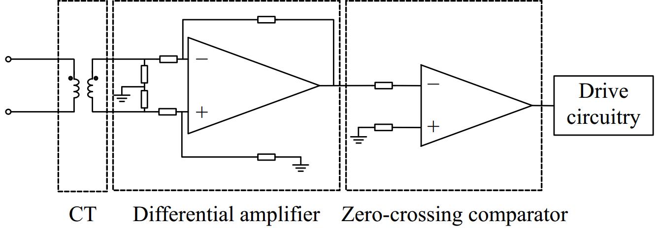
Figure 4.
Controller structure.
The core function of the controller is to actively regulate the output voltage phase based on current feedback, enabling adaptive steady-state adjustment of the system. The controller first samples the current of the primary-side resonant cavity using a current transformer. The sampled signal is then processed by a differential amplification circuit, converting the current signal into a voltage signal. Subsequently, this voltage signal is processed by a zero-crossing comparator to generate a square wave signal, which is then fed into the driver circuit to produce control signals for the switching devices. Overall, this control strategy effectively achieves phase regulation of the inverter's output voltage, thereby optimizing the system's dynamic response characteristics. In its specific operating mode, the system dynamically adjusts the switching states according to the current direction, ensuring that the inverter's output square wave voltage remains phase-aligned with the sinusoidal current. When i1 is greater than 0, S1 and S4 are turned on, when i1 is less than 0, S2, and S3 are turned on, and the zero current switch is realized, and the inverter output voltage is a square wave at this time. The phase of the voltage fundamental is the same as that of the inverter output current, and the characteristics of negative resistance are realized. At this time, the operating frequency of the system is approximately a certain frequency in f1, f2, and f3, and when the system parameters change, the system can adaptively maintain the characteristics of ZCS through frequency conversion.
-
As mentioned in the previous section, the voltage waveform after the full-bridge inverter is approximately a square wave, when the current crosses zero, the switching mode is switched, neglecting the parasitic parameters of the switching devices, and the nonlinear characteristics introduced by the inverter circuit can be equivalent to a reverse relay characteristic, then the system structure diagram can be equivalent to what is shown in Fig. 5, N(A) is its nonlinear component, A is the amplitude of the difference between the reference input and the feedback input, when the inverter output current is greater than 0, the bridge voltage output is Us, and when the output current is less than 0, the output voltage is flipped to −Us.
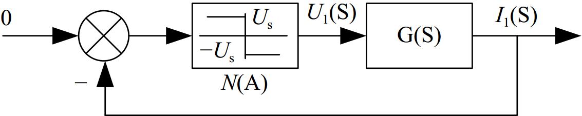
Figure 5.
Structure diagram of the system.
$ \left\{ \begin{gathered} G(S) = \dfrac{1}{{{Z_{{\text{in}}}}(S)}} \\ N(A) = - \dfrac{{4{U_{\text{s}}}}}{{\pi A}} \\ \end{gathered} \right. $ (8) Equivalence of the SS compensation network to a two-port network, there is:
$ \left( \begin{gathered} {U_1}(S) \\ {U_2}(S) \\ \end{gathered} \right) = \left( {\begin{array}{*{20}{c}} \begin{gathered} {Z_{11}}(S) \\ {Z_{21}}(S) \\ \end{gathered} &\begin{gathered} {Z_{12}}(S) \\ {Z_{22}}(S) \\ \end{gathered} \end{array}} \right)\left( \begin{gathered} {I_1}(S) \\ {I_2}(S) \\ \end{gathered} \right)$ (9) where,
$ \left( {\left. {\begin{array}{*{20}{c}} {{Z_{11}}(S)}&{{Z_{12}}(S)} \\ {{Z_{21}}(S)}&{{Z_{22}}(S)} \end{array}} \right)} \right. = \left( {\begin{array}{*{20}{c}} \begin{gathered} \dfrac{{1 + {C_1}{L_1}{S^2}}}{{{C_1}S}} + {R_1} \\ MS \\ \end{gathered} &\begin{gathered} MS \\ \dfrac{{1 + {C_2}{L_2}{S^2}}}{{{C_2}S}} + {R_2} \\ \end{gathered} \end{array}} \right) $ (10) Bringing U2(S) = −RLI2(S) into the above equation yields:
$ G(S) = \dfrac{{{I_1}(S)}}{{{U_1}(S)}} = \dfrac{1}{{{Z_{{\text{in}}}}(S)}} = \dfrac{{{Z_{22}}(S) + {R_{\text{L}}}}}{{{Z_{11}}(S){Z_{22}}(S) + {Z_{11}}(S){R_{\text{L}}} - {Z_{12}}(S){Z_{21}}(S)}} $ (11) There are three possible self-sustaining oscillation frequency points under the frequency bifurcation of the system, the system parameter settings are shown in Table 1, (a) C1 = C2 = 20 nF, (b) C1 = 22 nF, C2 = 20 nF, (c) C1 = 20 nF, C2 = 22 nF.
Table 1. System parameters.
Parameters Value Input voltage Us 10 V Primary side compensation capacitor C1 20.1 (22.2) nF Primary coil self-inductive L1 103.2 μH Secondary coil self-inductance L2 103.4 μH Secondary side compensation capacitor C2 20.0 (22.1) nF Equivalent load RL 20 Ω From the polar coordinate graph, it can be seen that the frequency corresponding to the intersection of the trajectories is the self-sustaining oscillation point of the system. Taking the imaginary part of G(jω), the expression of Eqn (3) can also be obtained. Solving Eqn (3) can obtain the corresponding frequency, and further determine the stable self-sustaining oscillation point of the system through the descriptive function method.
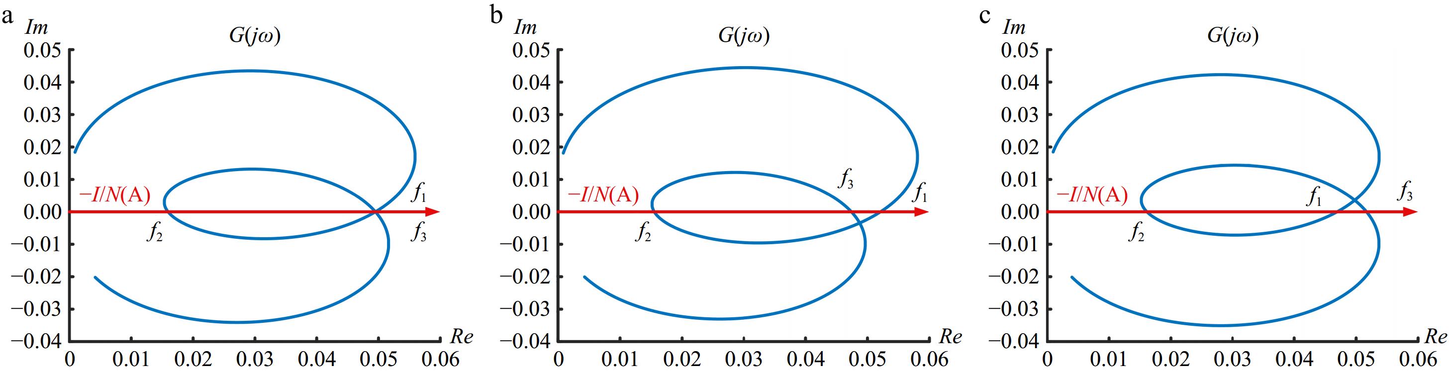
Figure 6.
Polar coordinate diagram. (a) ωp = ωs, (b) ωp < ωs, and (c) ωp > ωs.
Under theoretical conditions, f1 and f3 are the stable self-sustaining oscillation frequencies of the system, and the actual operating frequency of the system are related to the initial value of the system, while in the actual system, due to the unavoidable tolerance of the components, it is difficult to tune the natural oscillation frequency of the primary and secondary sides to the same frequency that is completely equal, and the existence of this difference leads to the unique determination of the stable operating frequency of the system, as shown in Fig. 6, when ωp < ωs, f1 is the stable operating frequency of the system, and when ωp > ωs, f3 is the stable operating frequency of the system.
Figure 7 shows the amplitude and frequency characteristics of the current in the two cases, at the operating frequency point, the maximum amplitude of the inverter output current of the system is obtained, which also corresponds to the point where the imaginary part of the system input admittance function is 0 and the real part is the largest in the polar graph.
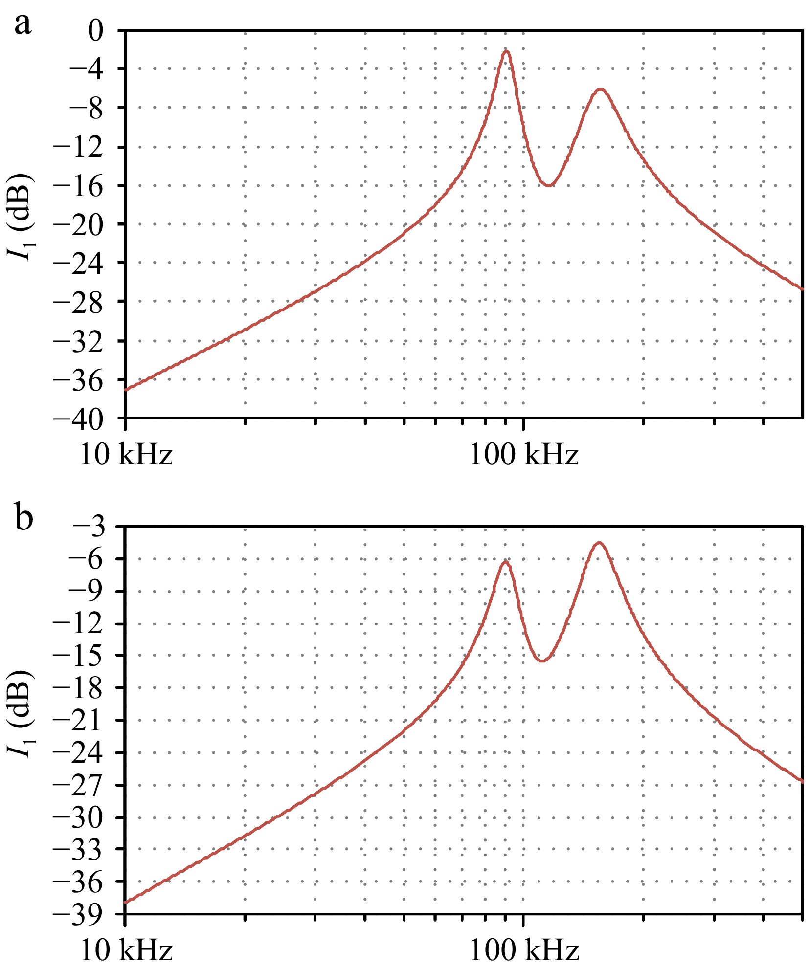
Figure 7.
Current amplitude frequency characteristics. (a) ωp < ωs, (b) ωp > ωs.
-
To verify the correctness of the mathematical model, an experimental setup as shown in Fig. 8 was built, and the system parameters are shown in Table 1.
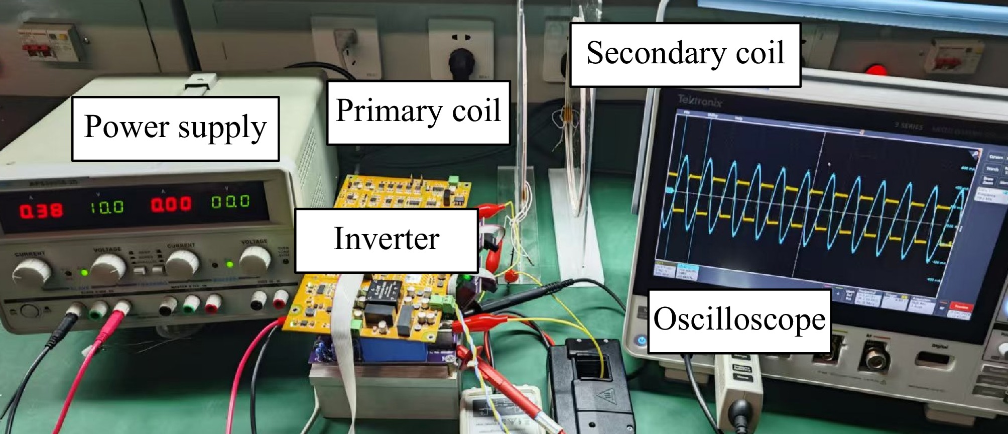
Figure 8.
Experimental device.
Figure 9 shows the waveform of the primary current and drive, and it can be observed that the switch state switches when the current crosses zero. This verification demonstrates the effectiveness of the current feedback controller in ensuring proper mode transitions. The results confirm that the system functions as an autonomous system, capable of naturally stabilizing into a periodic trajectory and exhibiting adaptive capabilities to maintain stable operation under varying conditions.
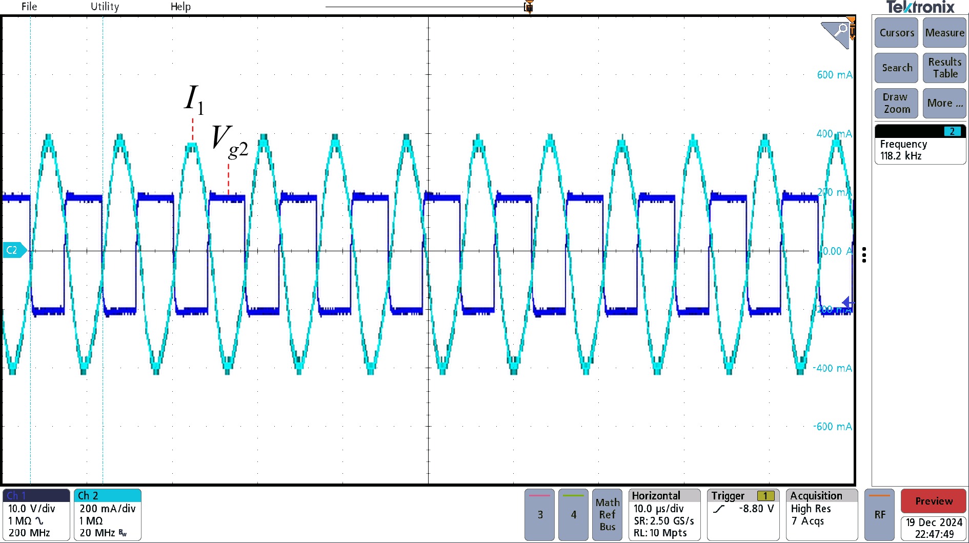
Figure 9.
Oscilloscope waveform.
When the system parameters change, the voltage and current waveform of the primary and secondary sides are shown in Fig. 10, this parameter adjustment is achieved by changing the spacing between the primary and secondary coils. As shown in the experimental setup in Fig. 8, adjusting the physical distance between the coils effectively alters the magnetic coupling strength between the primary and secondary sides, thereby modifying the coupling coefficient. When the resonant frequency changes due to the parameter change, the system can smoothly switch and adaptively adjust the operating frequency, to achieve stable operation. This primarily reflects the system's adaptive process, demonstrating its ability to adjust to parameter changes and reach a steady state.
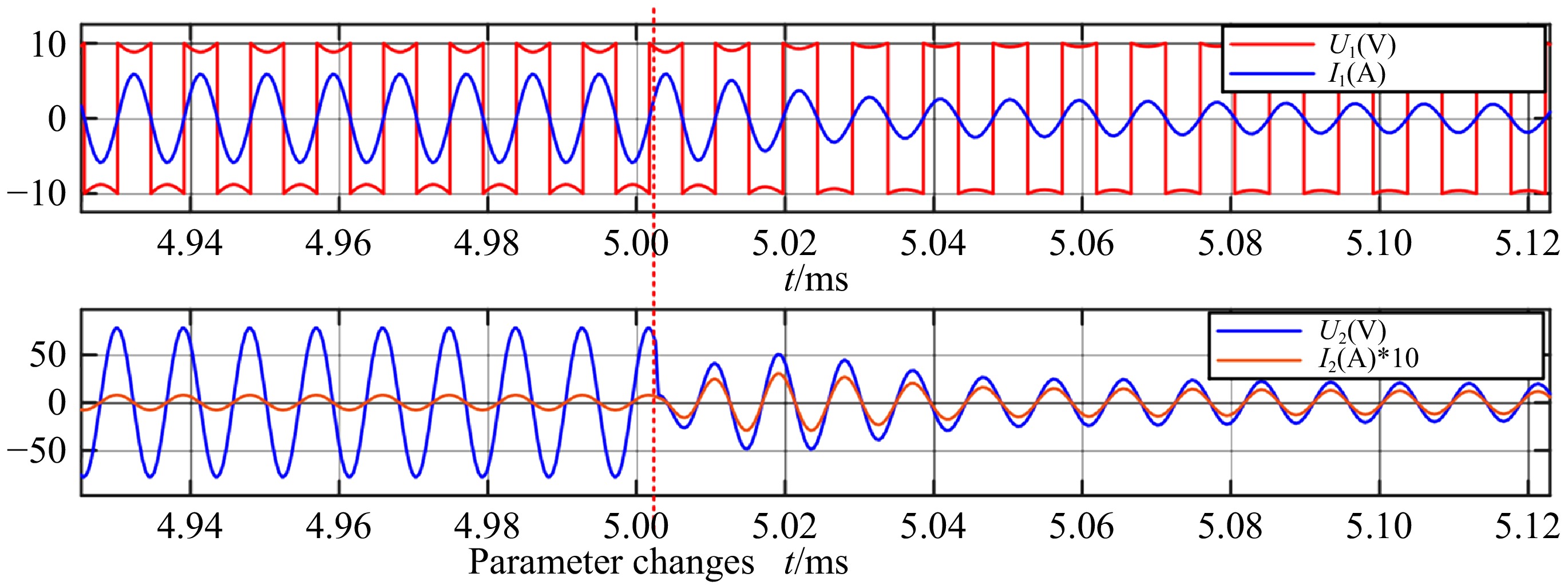
Figure 10.
Input and output waveforms during parameter changes.
By setting the compensation capacitance value of the primary and secondary sides, the experimental results shown in the following figure can be obtained by simulating the inconsistency of the system parameters under actual working conditions.
As shown in Figs 11 and 12, the actual operating frequency of the system is related to the natural oscillation frequency of the primary and secondary sides, which is consistent with the theoretical values calculated by the model, verifying the accuracy of the model in the previous section.
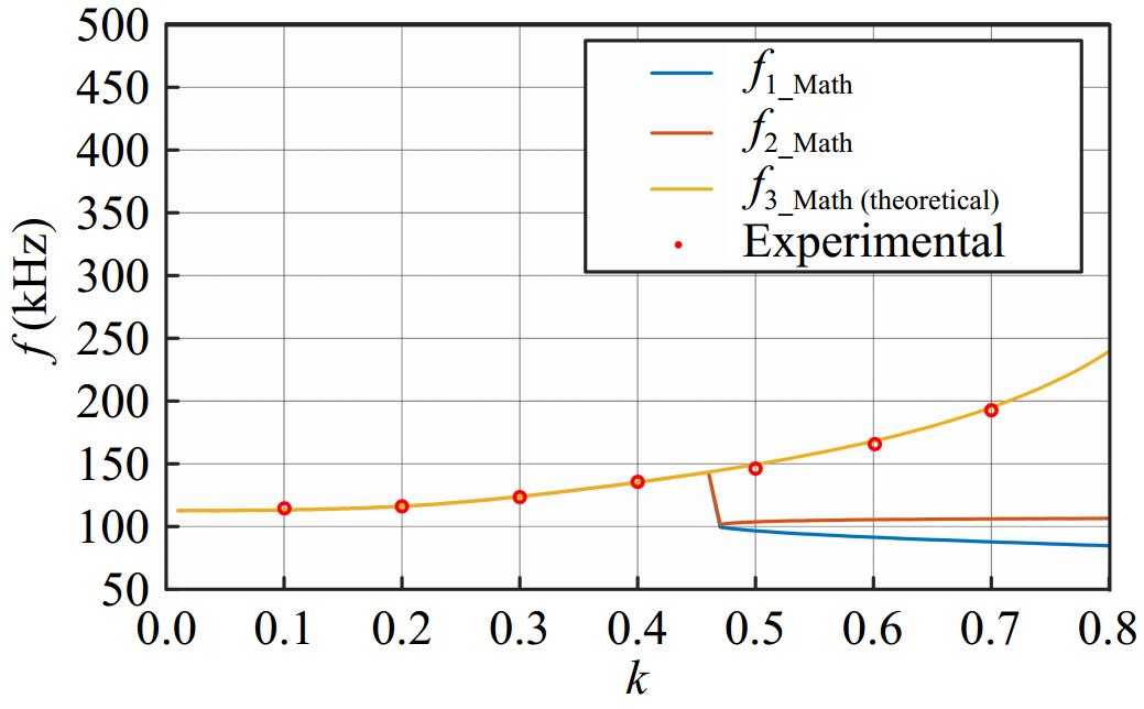
Figure 11.
Relationship between system operating frequency and coupling coefficient when ωp < ωs.
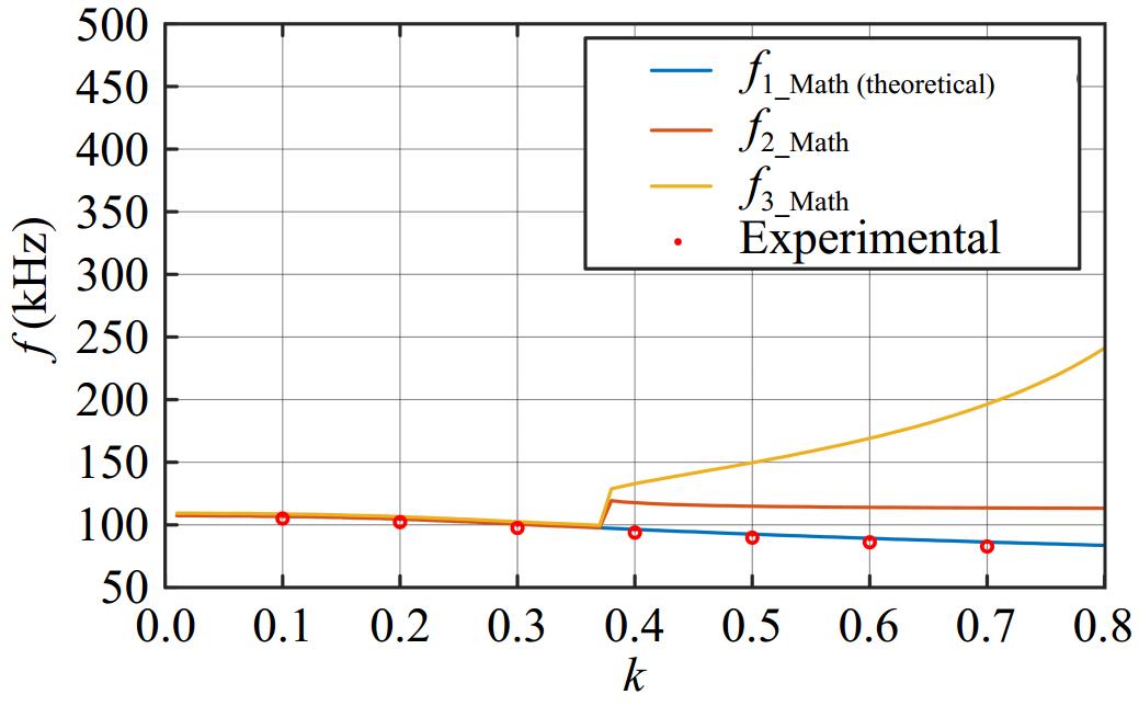
Figure 12.
Relationship between system operating frequency and coupling coefficient when ωp > ωs.
According to Eqn (3), the relationship between the frequency bifurcation point and the coupling coefficient of the system can be obtained by solving the cubic equation. The calculation shows that the coupling coefficients of 0.38 and 0.45 correspond to the critical bifurcation points in two cases, respectively. When the adaptive SS system is in the frequency bifurcation interval, the system can maintain relatively stable output characteristics, as shown in Fig. 13. The output of the constant pressure interval system does not change with the coupling coefficient and has good resistance to parameter offset.
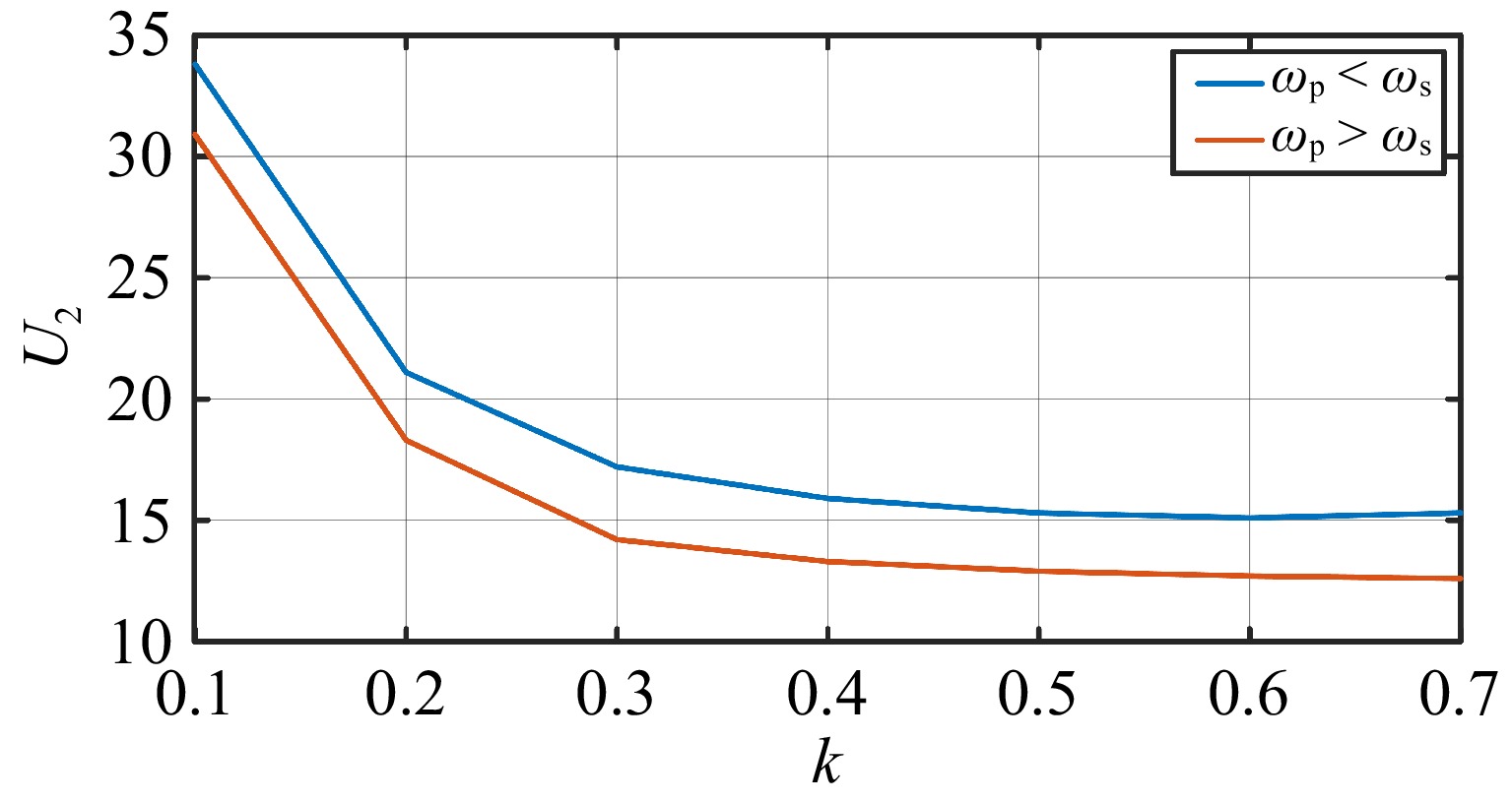
Figure 13.
Output voltage amplitude.
-
In this paper, the actual operating frequency of the frequency-adaptive SS compensation system is determined through model analysis, and its effectiveness is validated through experiments. The study establishes a mathematical model to predict the system's working frequency, demonstrating that the circuit can be approximated as a closed-loop negative feedback system with nonlinear links. By employing the describing function method, the stable self-sustained oscillation frequency during steady-state operation is derived, along with its relationship to system parameters. Furthermore, the model provides insights into the system's stable operating frequency under variations in the natural oscillation frequencies of the primary and secondary sides.
A key finding of this research is that at the bifurcation points, the system exhibits strong output robustness, and its input impedance remains invariant with respect to the coupling coefficient at both low and high-frequency points. This decouples the system from the coupling coefficient, enabling frequency adaptation through circuit design under parameter variations. The experimental results confirm the model's predictive accuracy in practical applications. However, due to the model's omission of switching device parasitic parameters and variations in coil self-inductance with frequency, discrepancies exist between the theoretical and actual operating frequencies. Additionally, the presence of parasitic capacitance in practical systems especially when using switching devices with high parasitic capacitance can alter the primary-side natural oscillation frequency, potentially shifting the system's actual operating frequency toward lower values. Under strong coupling conditions, the influence of higher harmonic components in the waveform increases[15], leading to deviations from the weak coupling scenario and necessitating further refinement of the model to account for parasitic parameters and nonlinearities in switching devices.
This study provides a theoretical foundation for designing frequency-adaptive wireless power transfer systems and highlights the necessity of improving mathematical models to better capture practical system behaviors, ensuring more accurate predictions and enhanced performance in real-world applications.
This work was supported by the Fundamental Research Funds for the Central Universities (Grant Nos 2022CDJQY-006, 2023CDJXY-011, and 2024CDJXY027).
-
The authors confirm their contributions to the paper as follows: study conception and design: Zeng W; data collection: Hang K, Chen X; analysis and interpretation of results: Zeng W, Dai X; draft manuscript preparation: Zhang W, Wu Y. All authors reviewed the results and approved the final version of the manuscript.
-
The datasets generated and analyzed during the current study are available from the corresponding author upon reasonable request.
-
The authors declare that they have no conflict of interest.
- Copyright: © 2025 by the author(s). Published by Maximum Academic Press, Fayetteville, GA. This article is an open access article distributed under Creative Commons Attribution License (CC BY 4.0), visit https://creativecommons.org/licenses/by/4.0/.
-
About this article
Cite this article
Zeng W, Hang K, Chen X, Zhang W, Wu Y, et al. 2025. Characteristic analysis of frequency adaptive SS compensation system. Wireless Power Transfer 12: e020 doi: 10.48130/wpt-0025-0015 

Characteristic analysis of frequency adaptive SS compensation system
- Received: 24 December 2024
- Revised: 03 April 2025
- Accepted: 28 April 2025
- Published online: 29 July 2025
Abstract: By analyzing the resonance frequency and frequency bifurcation characteristics of the wireless power transmission SS compensation system, the characteristic frequencies of the system with stable and strong output robustness are obtained at the frequency bifurcation, and the input impedance does not change with the coupling coefficient at the low-frequency point and the high-frequency point. The system is decoupled from the coupling coefficient, and the system can follow this frequency under the parameter change through the circuit design, to realize the frequency adaptation and a mathematical model to determine the working frequency of the system is established. This shows that the circuit can be approximated as a closed-loop negative feedback system with nonlinear links. Through the method of describing the function to determine the stability frequency of the system, the self-sustaining oscillation frequency of the system during stable operation is solved, the relationship between it and the system parameters is obtained, and the stable operating frequency of the system under the difference of the natural oscillation frequency of the primary and secondary sides is obtained according to the model, and the effectiveness of the model is verified by experiments.
-
Key words:
- Wireless power transfer