


-
With the widespread recognition of the concept of green communication, radio frequency energy harvesting (RF-EH) technology has gradually become a research hotspot[1,2]. A hybrid spectrum access mechanism integrating NOMA-based cooperative transmission and beamforming technology was proposed, with the outage probability of secondary users theoretically derived for the proposed mechanism[3]. A multi-input single-output (MISO) downlink communication system architecture based on Rate Splitting Multiple Access (RSMA) technology is proposed[4]. RSMA achieves optimal performance by decoding the information intended for the target user while treating the information of other users as noise. The selection of secure relays for device-to-device (D2D) communication in cellular networks was investigated[5]. By defining the closed form of the relay selection area in the D2D link and its interruption probability, a safe relay selection scheme using social relations as a safety factor for relay-assisted D2D communication systems is proposed.
Buffer-aided relays utilizing finite-size energy buffers to accumulate energy harvested from source signals were studied[6]. A relay selection scheme that considers the states of data buffer and energy buffer at the same time is proposed, and its performance is theoretically analyzed through the Markov chain model. Two energy and spectrum-efficient transmission strategies were proposed[7]. For the proposed WPT-NOMA scheme, considering the hybrid continuous interference cancellation (SIC) decoding sequence, it is proven that WPT-NOMA can avoid the error threshold of power failure probability and achieve full diversity gain. Unlike WPT-NOMA, BAC-NOMA has an error threshold for the probability of power failure, and the asymptotic behavior of the error threshold can be proved theoretically. Methods for improving performance indicators, including spectrum efficiency and system capacity, were studied[8]. A scenario to extend D2D communication technology to vehicular infrastructure was proposed. The performance of the TLE frequency band for vehicular traffic was analyzed and network simulation was performed.
A nonlinear recursive model was proposed for energy harvesting communication networks, enabling effective simulation of the collected energy transmission process in real-world environments[9]. A new media access control (MAC) protocol was introduced[10]. Devices in a WLAN with 802.11 IEEE Distributed Coordination Function (DCF) can use the remaining energy to selectively execute energy transmission requests, which can minimize the network throughput. The energy efficiency (EE) maximization problem in RF-EH heterogeneous cellular networks (HetNets) was investigated[11]. Considering the fairness of users when allocating resources, the problem of maximizing network EE is reduced to a hybrid combination and non-convex optimization problem. The impacts of energy efficiency, delay, and random data arrival on system performance were discussed[12]. A resource allocation model for wireless mobile edge computing (MEC) scenarios was established and an online computing offloading method proposed based on random channels and Lyapunov theory.
This paper investigates an RF-EH multi-relay cooperative communication network. By adopting the improved hybrid time switching (HTC) protocol, the base station transfers energy to the source node and relays during the energy transmission phase. In the data transmission stage, the source node first sends signals to both relays and the base station simultaneously in the first time slot. In the second time slot, all relays forward the received signals to the base station, while the source node retransmits its first-slot signals. This retransmission mechanism is designed to enhance system reliability by leveraging spatial diversity.
A joint optimization model is formulated to maximize the average EE under practical constraints, considering optimal power allocation, subcarrier pairing, and time slot assignment. The problem is a mixed-integer nonlinear programming (MINLP) issue with high computational complexity, intractable for conventional solvers. To address this, a nonlinear programming model of the objective function is first established, which is linearized via the Dinkelbach method. The Hungarian algorithm is then employed to iteratively tackle the joint resource allocation problem. Finally, an iterative algorithm combining dual decomposition and subgradient methods is used to derive the optimal EE solution. Part of this work was previously presented at the EAI BROADNETS 2020 conference[13].
The main contributions of this paper are as follows:
(1) A three-phase energy harvesting cooperative communication protocol is proposed, allowing the source node to transmit data twice. This enables relays and the source to harvest sufficient energy for collaboration, ultimately achieving higher system diversity gain.
(2) An optimal EE-oriented joint resource allocation model is established, integrating subcarrier pairing, power allocation, and time slot assignment in a complex scenario while prioritizing energy efficiency maximization.
(3) For the NP-hard problem, an iterative optimization algorithm based on the Dinkelbach method is developed to reduce computational complexity. The Hungarian algorithm ensures rapid convergence to the optimal joint resource allocation solution.
-
An HTC protocol was presented for a three-node relay scenario[14]. The source node and the relay node harvest energy from the HAP in the downlink and then use the collected energy to assist the source node's information transmission. A closed-form expression of the delay-constrained average throughput under the Rayleigh channel condition of the protocol is proposed, and an asymptotic analysis of the approximate throughput under the multi-relay HTC scheme is given. An energy-efficient hybrid energy harvesting system was developed, which harvests energy from solar, vibration, and radio frequency (RF) sources. The distribution problem of RF energy harvesting was further explored[15]. A resource allocation strategy for drone-assisted edge computing in a wireless power communication network was studied[16]. By jointly optimizing factors such as power and time, the optimal system performance was achieved.
The resource allocation problem in a wireless power communication network (WPCN) with a hybrid access point (HAP), and two energy harvesting users was investigated[17]. Using the HTC-based user cooperation protocol, the user close to the HAP uses the collected energy and allocated time to provide relay services for another user. Considering user quality of service (QoS) requirements and fairness, the total throughput of WPCN is maximized. The optimal configuration of parameters for the NOMA-based IoT relay system was explored[18]. The key indicators, such as EH time and NOMA coefficients are mainly studied. A wireless communication system with a relay was considered[19]. Aiming at maximizing the network throughput, a new optimization problem is proposed. Solving the optimization problem can jointly optimize the ratio of transmission energy and signal power over time. A hybrid relay scheme was proposed, realized by a self-sustaining intelligent reflector (IRS) in a WPCN[20]. For TS and power allocation (PS) schemes, the problem of maximizing the sum is proposed by jointly optimizing the phase shift of IRS and network resource allocation. Relay selection schemes in energy harvesting wireless sensor networks were discussed[21]. To take into account the requirements of transmission delay and energy efficiency, a relay selection scheme based on reinforcement learning is proposed. Considering that there may be eavesdroppers in the communication process between two users, it is necessary to carry out secret communication between users. A secure two-way relay scheme based on time-division broadcasting was proposed[22]. Under the constraints of average peak transmit power and data buffer, a safe total rate maximization problem is proposed. Different model predictive control was studied to optimize HEV nonlinear energy management to achieve better fuel economy[23]. By treating MPC as a non-linear programming problem, using sequential secondary programming to obtain the descending direction of the control variable, the current control input is obtained. The control strategy for edge nodes with caching capabilities was studied, a dynamic programming model based on truncation concepts was established, and an asymptotically optimal algorithm was proposed[24]. The resource allocation problem in a reconfigurable smart surface-assisted wireless power transfer system was studied[25]. To deal with the beamforming optimization model, a scheme based on alternating direction multipliers was proposed to perform the beamforming optimization algorithm.
-
As shown in Fig. 1, the system model includes a base station B, a source node S, and K AF relays {Rk, k = 1, 2, ..., K}. The node S and all relays can collect energy from the entire transmission bandwidth, which is divided evenly into N sub-carriers. The base station has a stable energy source to guarantee communication. hBS and PB represent the channel gain and transmission power of BS.
$ h_k^{BR} $ 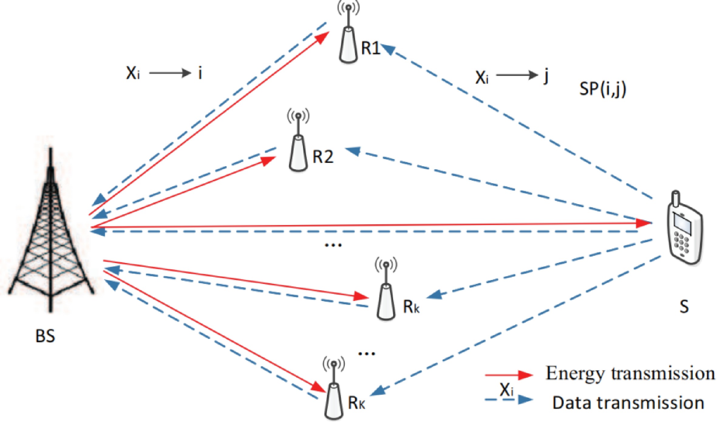
Figure 1.
Multi-relay network with an RF-EH scenario.
As shown in Fig. 2, in the energy transmission phase
$ {\tau} $ 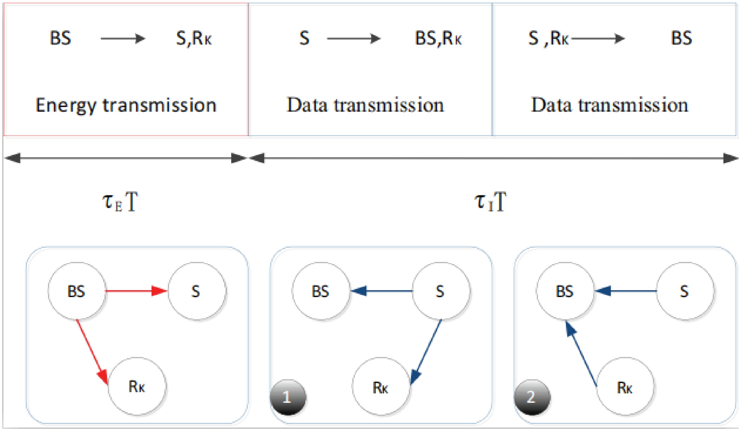
Figure 2.
Improved HTC protocol.
$ {E^S} = {\zeta _S}{\tau _E}T{h^{BS}}{P_B} $ (1) $ E_k^R = \zeta _k^R{\tau _E}Th_k^{BR}{P_B}, k \in \left\{ {1,2,...,K} \right\} $ (2) $ {E^{EH}} = {\tau _E}T\left( {{\zeta _S}{h^{BS}} + \sum\limits_{k = 1}^K {\zeta _k^Rh_k^{BR}} } \right){P_B} $ (3) where,
$ {\zeta _S} $ $ \zeta _k^R $ $ {\Phi _{N{\text{x}}N}} = \left\{ {{\phi _{i,j}}} \right\} $ $ {\phi _{i,j}} \in \{ 0,1\} ,\forall i,j $ (4) $ \sum\limits_{i = 1}^N {{\phi _{i,j}}} = 1,\sum\limits_{j = 1}^N {{\phi _{i,j}}} = 1,\forall i,j $ (5) The signals received by the k-th relay and BS at the subcarrier i are represented as
$ y_{i,k}^R $ $ y_i^B $ $ g_{i,{\text{1}}}^{SB} $ $ g_{i,k}^{SR} $ $ y_{i,k}^R = g_{i,k}^{SR}\sqrt {P_i^{S{\text{1}}}} {x_i} + n_{i,k}^{SR}, \forall i,k $ (6) $ y_i^B = g_{i,{\text{1}}}^{SB}\sqrt {P_i^{S{\text{1}}}} {x_i} + n_{i,{\text{1}}}^{SB}, \forall i $ (7) For the SPi,j, the received joint signal
$ y_{(i,j)}^B $ $ y_{(i,j)}^B = g_{j,{\text{2}}}^{SB}\sqrt {P_{i,j}^{S{\text{2}}}} {x_i} + \sum\limits_{k = 1}^K {g_{j,k}^{RB}\alpha _{i,k}^R} y_{i,k}^R + n_{j,{\text{2}}}^{SB} $ (8) Further, the SNR in the first and second time slots are:
$ SNR_{(i,j)}^{TS{\text{2}}} = \dfrac{{{{\left( {\displaystyle\sum\limits_{k = 1}^K {\dfrac{{\left| {g_{j,k}^{SR}g_{j,k}^{RB}} \right|\sqrt {P_i^{S{\text{1}}}P_{i,j,k}^R} }}{{\sqrt {P_i^{S{\text{1}}}{{\left| {g_{j,k}^{SR}} \right|}^2} + \sigma _{SR,k}^2} }} + \left| {g_{j,2}^{SB}} \right|\sqrt {P_{i,j}^{S2}} } } \right)}^2}}}{{\sigma _{SB,2}^2 + \displaystyle\sum\limits_{k = 1}^K {{{\left( {\dfrac{{\left| {g_{j,k}^{RB}} \right|\sqrt {P_{i,j,k}^R} }}{{\sqrt {P_i^{S1}{{\left| {g_{j,k}^{SR}} \right|}^2} + \sigma _{SR,k}^2} }}} \right)}^2}\sigma _{SR,k}^2} }} $ (9) $ SNR_i^{TS{\text{1}}} = {\left| {g_{i,{\text{1}}}^{SB}} \right|^2}P_i^{S{\text{1}}}/\sigma _{SB,{\text{1}}}^2 $ (10) where:
$ \alpha _{i,k}^R = \sqrt {P_{i,j,k}^R{\text{ }}/\left( {{{\left| {g_{i,k}^{SR}} \right|}^2}P_i^{S{\text{1}}} + \sigma _{R,k}^2} \right)} $ (11) Problem description
-
Therefore, we have the end-to-end transmission rate R(i,j) and the total reachable rate
$ {R_{total}}({\mathbf{\Phi }},{\mathbf{P}}) $ $ {R_{(i,j)}} = \dfrac{{{\tau _I}}}{2}\log (1 + SNR_i^{TS1} + SNR_{(i,j)}^{TS2}) $ (12) $ {R_{total}}({\mathbf{\Phi }},{\mathbf{P}}) = \sum\limits_{i = 1}^N {\sum\limits_{j = 1}^N {{\phi _{i,j}}} } {R_{(i,j)}} $ (13) where,
$ {\mathbf{\Phi }} = \left\{ {{\phi _{i,j}}} \right\},{\mathbf{P}} = \left\{ {{P_{i,j}}} \right\} $ $ {P_{trans}}({\mathbf{\Phi }},{\mathbf{P}}) = \sum\limits_{i = 1}^N {\sum\limits_{j = 1}^N {\left( {P_i^{S1} + P_{i,j}^{S2}} \right)} } + \sum\limits_{i = 1}^N {\sum\limits_{j = 1}^N {P_{i,j,k}^R} } = \sum\limits_{i = 1}^N {\sum\limits_{j = 1}^N {{\phi _{i,j}}{P_{\left( {i,j} \right)}}} } $ (14) $ {P_{total}}({\mathbf{\Phi }},{\mathbf{P}}) = {P_C} + \varsigma {P_{trans}}({\mathbf{\Phi }},{\mathbf{P}}) $ (15) The scenario considered in this paper is joint resource optimization which must meet the constraints as follows:
$ \sum\limits_{i = 1}^N {\sum\limits_{j = 1}^N {\left( {P_i^{S1} + P_{i,j}^{S2}} \right)} } \leq {P^S} = \dfrac{{1 - {\tau _I}}}{{{\tau _I}}}2{\zeta _S}{h^{BS}}{P_B} $ (16) $ \sum\limits_{i = 1}^N {\sum\limits_{j = 1}^N {\sum\limits_{k = 1}^K {P_{i,j,k}^R} } } \leq \sum\limits_{k = 1}^K {P_k^R} = \dfrac{{1 - {\tau _I}}}{{{\tau _I}}}2\zeta _k^R{P_B}\sum\limits_{k = 1}^K {h_k^{BR}} $ (17) where, PS represents the sum power of S in the communication slots,
$ P_k^R $ $ \sum\limits_{i = 1}^N {\sum\limits_{j = 1}^N {{\phi _{i,j}}} } {P_{i,j}} = {P^S} + \sum\limits_{k = 1}^K {P_k^R} \leq {P_T} $ (18) Therefore, the EE optimization problem is modeled as:
$ \begin{aligned} P1:\;\;&\mathop {\max }\limits_{{\tau _I},P_i^{S{\text{1}}},P_{i,j}^{S{\text{2}}},P_{i,j,k}^R,{\phi _{i,j}}} \dfrac{{{R_{total}}({\mathbf{\Phi }},{\mathbf{P}})}}{{{P_{total}}({\mathbf{\Phi }},{\mathbf{P}})}} \\ &s.t. {\phi _{i,j}} \in \{ 0,1\} ,\forall i,j \end{aligned} $ (19A) $ \quad\quad \sum\limits_{i = 1}^N {{\phi _{i,j}}} = 1,\sum\limits_{j = 1}^N {{\phi _{i,j}}} = 1,\forall i,j $ (19B) $\quad\quad \sum\limits_{i = 1}^N {\sum\limits_{j = 1}^N {\left( {P_i^{S1} + P_{i,j}^{S2}} \right)} } \leq {P^S} = \dfrac{{1 - {\tau _I}}}{{{\tau _I}}}2{\zeta _S}{h^{BS}}{P_B} $ (19C) $ \quad\quad \sum\limits_{i = 1}^N {\sum\limits_{j = 1}^N {\sum\limits_{k = 1}^K {P_{i,j,k}^R} } } \leq \sum\limits_{k = 1}^K {P_k^R} = \dfrac{{1 - {\tau _I}}}{{{\tau _I}}}2{P_B}\sum\limits_{k = 1}^K {\zeta _k^Rh_k^{BR}} $ (19D) $\quad\quad\sum\limits_{i = 1}^N {\sum\limits_{j = 1}^N {{\phi _{i,j}}} } {P_{i,j}} = {P^S} + \sum\limits_{k = 1}^K {P_k^R} \leq {P_T} $ (19E) R(i,j) represents the transmission rate between endpoints, and ϕi,j represents the carrier pairing factor on the carrier pair SPi,j. The first two constraints refer to the fact that one subcarrier has and only one subcarrier is paired with it. The last three constraints are the energy rate constraints for the three terminal nodes. The resulting optimization problem is an NP-hard problem, which needs to be solved by the interior point method with high computational complexity.
-
The P1 is a MINLP problem that needs the Dinkelbach method to solve it. The Dinkelbach algorithm is an effective algorithm for solving fractional programming problems. The algorithm solves the fractional programming problem by converting it into a series of parameterized sub-problems. The core of the algorithm is to find the optimal solution in an iterative way. The Dinkelbach algorithm can ensure that the optimal solution of the problem is reached within a finite number of steps, thanks to its unique parameter update mechanism and convergence properties.
By scaling Eq. (4), P1 can be transformed into a quasi-convex form[26].
$ {\phi _{i,j}} \in \left[ {0,1} \right],\forall i,j $ (20) $ \begin{aligned} P2:\;\;\;\;\;\;\;\;\;& \mathop {\max }\limits_{{\tau _I},P_i^{S{\text{1}}},P_{i,j}^{S{\text{2}}},P_{i,j,k}^R,{\phi _{i,j}}} \dfrac{{{R_{total}}({\mathbf{\Phi }},{\mathbf{P}})}}{{{P_{total}}({\mathbf{\Phi }},{\mathbf{P}})}} \\ &s.t. {\phi _{i,j}} \in \left[ {0,1} \right],\forall i,j \\ &\qquad(19B) - (19E) \end{aligned} $ (21) Lemma 1. The relaxation problem P2 has the same optimal solution as the original problem P1.
Proof of Lemma 1. It is not difficult to find that the value range of the constraint ϕi,j
$ \in $ $ \in $ $ \left( {{{\mathbf{\Phi }}^*},{{\mathbf{P}}^*}} \right) $ $ {{\mathbf{\Phi }}^*}\left( {\alpha ,\beta } \right) $ $ \left( {{{\mathbf{\Phi }}^*},{{\mathbf{P}}^*}} \right) $ Dinkelbach method and its outer loop algorithm
-
Adopting the Dinkelbach method
$ {\eta ^*} = \mathop {\max }\limits_{{\mathbf{\Phi }},{\mathbf{P}}} \dfrac{{{R_{total}}({\mathbf{\Phi }},{\mathbf{P}})}}{{{P_{total}}({\mathbf{\Phi }},{\mathbf{P}})}} = \dfrac{{{R_{total}}({{\mathbf{\Phi }}^*},{{\mathbf{P}}^*})}}{{{P_{total}}({{\mathbf{\Phi }}^*},{{\mathbf{P}}^*})}},\forall \{ {\mathbf{\Phi }},{\mathbf{P}}\} \in {\mathbf{T}} $ (22) Define function
$ F(\eta ) $ $ F(\eta ) = \mathop {\max }\limits_{{\mathbf{\Phi }},{\mathbf{P}}} \left[ {{R_{total}}({\mathbf{\Phi }},{\mathbf{P}}) - \eta {P_{total}}({\mathbf{\Phi }},{\mathbf{P}})} \right] $ (23) Proposition 1. According to Eqs (22), (23), the sufficient and necessary conditions for the optimization problem P2 to obtain the optimal solution
$ \left\{ {{\eta ^*},{{\mathbf{\Phi }}^*},{{\mathbf{P}}^*}} \right\} $ $ \begin{aligned} F({\eta ^*}) & = \mathop {\max }\limits_{{\mathbf{\Phi }},{\mathbf{P}}} \left[ {{R_{total}}({\mathbf{\Phi }},{\mathbf{P}}) - {\eta ^*}{P_{total}}({\mathbf{\Phi }},{\mathbf{P}})} \right] \\ & = {R_{total}}({{\mathbf{\Phi }}^*},{{\mathbf{P}}^*}) - {\eta ^*}{P_{total}}({{\mathbf{\Phi }}^*},{{\mathbf{P}}^*}) = 0,\forall \{ {\mathbf{\Phi }},{\mathbf{P}}\} \in {\text{T}} \end{aligned} $ (24) Proof of Proposition 1. First, the optimization problem P2 is reduced to a fractional programming problem, and its optimal energy efficiency value is
$ {\eta ^*} = \frac{{{R_{total}}({{\mathbf{\Phi }}^*},{{\mathbf{P}}^*})}}{{{P_{total}}({{\mathbf{\Phi }}^*},{{\mathbf{P}}^*})}} $ $ {P_{total}}({\mathbf{\Phi }},{\mathbf{P}}) = {P_C} + \varsigma \sum\limits_{m = 1}^N {\sum\limits_{n = 1}^N {{P_{i,j}}} } $ $ {P_C} $ $ \varsigma $ In summary, the denominator polynomial
$ {P_{total}}({\mathbf{\Phi }},{\mathbf{P}}) $ $ {R_{total}}({\mathbf{\Phi }},{\mathbf{P}}) $ According to Eq. (22), the Dinkelbach method can achieve optimal energy efficiency
$ {\eta ^*} $ $ {\mathbf{P}} $ $ {\mathbf{\Phi }} $ Lemma 2. For
$ \forall \{ \Phi ',{{\text{P}}^\prime }\} \in {\text{T}} $ $ \eta ' = {\eta _E}(\Phi ',{{\text{P}}^\prime }) $ $ F(\eta ') \geqslant 0 $ $ \eta ' = {\eta ^*} $ $ F(\eta ') = 0 $ $ F(\eta ') = \mathop {\max }\limits_{{\mathbf{t}},{\mathbf{P}}} \left[ {{R_{total}}(\Phi ,{\text{P}}) - \eta '{P_{total}}(\Phi ,{\text{P}})} \right] \geqslant {R_{total}}(\Phi ',{{\text{P}}^\prime }) - \eta '{P_{total}}(\Phi ',{{\text{P}}^\prime }) = 0 $ (25) Proposition 2. The sequence {ηn} generated by Algorithm 1 is a convergent sequence, and the convergence value ηlmt is reachable.
Table 1. Energy efficiency optimization iterative algorithm.
1. Initialize. 2. Set the iteration termination times $ N_{outer}^{max} $, iteration termination accuracy $ {\varpi }_{outer} $, and the initial iteration value $ {\eta }_{0}=0 $ and $ n=0 $. 3. Loop body: 4. Update iteration index $ n=n+1 $. 5. Solving the Optimization Problem $ F({\eta }_{n-1})=\underset{\mathbf{\Phi },\mathbf{P}}{\max }\left[{R}_{total}(\mathbf{\Phi },\boldsymbol{P})-{\eta }_{n-1}{\mathbf{P}}_{total}(\mathbf{\Phi },\mathbf{P})\right] $, gain $ \left\{{\mathbf{\Phi }}^{*},{\mathbf{P}}^{*}\right\} $. 6. Calculate the energy efficiency under the current iterative index using $ \left\{{\mathbf{\Phi }}^{*},{\mathbf{P}}^{*}\right\} $, $ {\eta }_{n}={R}_{total}({\mathbf{\Phi }}^{*},{\boldsymbol{P}}^{\text{*}})/{\mathbf{P}}_{total}({\mathbf{\Phi }}^{*},{\mathbf{P}}^{*}) $. 7. End Condition: $ \left| {\eta }_{n}-{\eta }_{n-1}\right| < {\varpi }_{outer} $ or $ n > N_{outer}^{max} $. 8. Output optimal solution $ \left\{{\eta }^{*},{\mathbf{\Phi }}^{*},{\mathbf{P}}^{*}\right\} $. Proof of Proposition 2. We first discuss the monotonicity of the sequence {ηn}. In order not to lose the generality, arbitrarily choose the n-th iteration, and solve the energy efficiency value of the
$ n $ $ {\eta _{n + 1}} = \dfrac{{{R_{total}}({\Phi _n},{{\text{P}}_n})}}{{{P_{total}}({\Phi _n},{{\text{P}}_n})}} $ (26) It is assumed that ηn and ηn+1have not yet reached the convergence value ηlmt of the energy efficiency sequence, namely ηn,ηn+1 ≠ ηlmt. According to Lemma 2, F(ηn) > 0, according to Eq. (25), expands as follows
$ \begin{aligned} F({\eta _n}) & = {R_{total}}({\Phi _n},{{\text{P}}_n}) - {\eta _n}{P_{total}}({\Phi _n},{{\text{P}}_n}) = {\eta _{n + 1}}{P_{total}}({\Phi _n},{{\text{P}}_n}) \\ & - {\eta _n}{P_{total}}({\Phi _n},{{\text{P}}_n}) = {P_{total}}({\Phi _n},{{\text{P}}_n})({\eta _{n + 1}} - {\eta _n}) \gt 0 \end{aligned} $ (27) The total power consumption
$ {P_{total}}({\Phi _n},{{\text{P}}_n}) $ The total power consumption of the system is
$ {P_{total}}({\Phi _n},{{\text{P}}_n}) = {P_C} + \varsigma \sum\limits_{m = 1}^N {\sum\limits_{n = 1}^N {{{\text{P}}_{i,j}}} } $ $ {P_{total}}({\Phi _n},{{\text{P}}_n}) $ $ \dfrac{{{R_{max}}}}{{{P_C}}} = {\eta ^{ub}} $ (28) Therefore, the non-negative sequence {ηn} increases monotonically, and there is an upper bound ηub, so the sequence {ηn} must converge, and the convergence value is ηlmt, which satisfies the following formula:
$ \begin{aligned} F({\eta ^{lmt}}) & = \mathop {\lim }\limits_{n \to \infty } F({\eta _n}) = \mathop {\lim }\limits_{n \to \infty } \mathop {\max }\limits_{{\mathbf{t}},{\mathbf{P}}} \left[ {{R_{total}}(\Phi ,{\text{P}}) - {\eta _n}{P_{total}}(\Phi ,{\text{P}})} \right] \\ &= \mathop {\lim }\limits_{n \to \infty } \mathop {\max }\limits_{{\mathbf{t}},{\mathbf{P}}} \left[ {{\eta _{n + 1}}{P_{total}}({\Phi _n},{{\text{P}}_n}) - {\eta _n}{P_{total}}(\Phi ,{\text{P}})} \right] \\ & = \mathop {\lim }\limits_{n \to \infty } ({\eta _{n + 1}} - {\eta _n}){P_{total}}({\Phi _n},{{\text{P}}_n}) = 0 \end{aligned} $ (29) In summary, the sequence {ηn} converges to ηlmt, and Proposition 2 is proved. The P2 is converted into other forms and solved by using a progressive optimization method in the following content.
-
This section presents a solution method for the inner loop optimization problem
$ F({\eta _{i - 1}}) $ $ P3:\mathop {\max }\limits_{ {\mathbf{\Phi }},{\mathbf{P}}} F(\eta ) = \left[ {{R_{total}}({\mathbf{\Phi }},{\mathbf{P}}) - \eta {P_{total}}({\mathbf{\Phi }},{\mathbf{P}})} \right] $ (30) Equivalent channel gain and optimization problem conversion
-
The total power consumption defined on the subcarriers SPi,j of the first and the second time slot is
$ P_{\left( {i,j} \right)}^{TS1} $ $ P_{\left( {i,j} \right)}^{TS2} $ $ {P_{(i,j)}} = P_{(i,j)}^{TS1} + P_{(i,j)}^{TS2} $ (31) The first time slot source S of information transmission sends data, and the second time slot K relay of information transmission simultaneously forwards data. In the improved transmission protocol of this article, the second time slot source S uses the collected excess energy to send data again. To increase the diversity gain, the power relationship is as follows:
$ P_{(i,j)}^{TS1} = P_i^{S1} $ (32) $ P_{(i,j)}^{TS2} = P_{i,j}^{S2} + \sum\limits_{k = 1}^K {P_{i,j,k}^R} ,\;\;\;\;\;\;\;P_{i,j}^{S2} \geq 0,P_{i,j,k}^R \geq 0 $ (33) To obtain the power allocation based on Eq. (33), it is necessary to simplify P(i,j) in Eq. (31) and obtain the equivalent channel gain of the system, which will help the subcarrier pairing in the following content. The definition is as follows:
$ P_{(i,j)}^{TS1} = {\varepsilon _{(i,j)}}{P_{(i,j)}},{\varepsilon _{(i,j)}} \in (0,1] $ (34) $ P_{(i,j)}^{TS2} = (1 - {\varepsilon _{(i,j)}}){P_{(i,j)}} $ (35) where, ε(i, j) represents the ratio of
$ P_{(i,j)}^{TS1} $ $ P_{(i,j)}^{TS2} $ Since Eqs (34) and (35) are both functions of P(i,j), we have:
$ SN{R_{(i,j)}} \approx {A_{(i,j)}}{P_{(i,j)}} $ (36) where, SNR(i, j) is the signal-to-interference and noise ratio of the subcarrier to SP(i, j). A(i, j) represents the equivalent channel gain of the subcarrier to SP(i, j). A(i, j) can be used to further optimize the simplified end-to-end transmission rate expression. A(i, j) can be expressed as:
$ {A_{(i,j)}} = \dfrac{1}{{{N_0}}}[{\left| {g_{j,2}^{SB}} \right|^2} + {\varepsilon _{(i,j)}}({\left| {g_{i,1}^{SB}} \right|^2} - {\left| {g_{j,2}^{SB}} \right|^2}) + \sum\limits_{k = 1}^K {\dfrac{{{\varepsilon _{(i,j)}}(1 - {\varepsilon _{(i,j)}}){{\left| {g_{i,k}^{SR}} \right|}^2}{{\left| {g_{j,k}^{RB}} \right|}^2}}}{{{\varepsilon _{(i,j)}}{{\left| {g_{i,k}^{SR}} \right|}^2} + (1 - {\varepsilon _{(i,j)}}){{\left| {g_{j,k}^{RB}} \right|}^2}}}} ] $ (37) According to Eq. (37) and the golden section method, the optimal solution of ε(i, j) can be obtained.
$ \varepsilon _{(i.j)}^* = \arg \max {A_{(i,j)}} $ (38) Power allocation and subcarrier pairing
-
Rewriting the expression of
$ SNR_{(i,j)}^{TS2} $ $ SNR_{(i,j)}^{TS2} = \dfrac{{P_i^{S1}}}{{{N_0}}}\cdot\dfrac{{{{\left( {\displaystyle\sum\limits_{k = 1}^K {\dfrac{{\left| {g_{i,k}^{SR}g_{j,k}^{RB}} \right|\sqrt {P_{i,j,k}^R} }}{{\sqrt {P_i^{S1}{{\left| {g_{i,k}^{SR}} \right|}^2} + {N_0}} }} + \left| {g_{j,2}^{SB}} \right|\sqrt {\dfrac{{P_{i,j}^{S2}}}{{P_i^{S1}}}} } } \right)}^2}}}{{1 + \displaystyle\sum\limits_{k = 1}^K {\dfrac{{{{\left| {g_{j,k}^{RB}} \right|}^2}P_{i,j,k}^R}}{{P_i^{S1}{{\left| {g_{i,k}^{SR}} \right|}^2} + {N_0}}}} }} $ (39) $ P_{i,j,k}^R $ $ P_{i,j}^{S2} $ $ P_{i,j,k}^R = \dfrac{{{{\left| {g_{i,k}^{SR}g_{j,k}^{RB}} \right|}^2}\theta _{i,j}^k}}{{\left( {\dfrac{{{{\left| {g_{j,k}^{RB}} \right|}^2}}}{{P_i^{S1}}} + \displaystyle\sum\limits_{k = 1}^K {\dfrac{{{{\left| {g_{i,k}^{SR}g_{j,k}^{RB}} \right|}^2}\theta _{i,j}^k}}{{{{(1 + \theta _{i,j}^k{{\left| {g_{j,k}^{RB}} \right|}^2}P_{i,j}^{S2})}^2}}}} } \right){{\left( {\dfrac{1}{{\sqrt {P_{i,j}^{S2}} }} + \theta _{i,j}^k{{\left| {g_{j,k}^{RB}} \right|}^2}\sqrt {P_{i,j}^{S2}} } \right)}^2}}} $ (40) $ P_{i,j}^{S2} = P_{\left( {i,j} \right)}^{TS2}{\left| {g_{j,2}^{SB}} \right|^2}/\left( {{{\left| {g_{j,k}^{RB}} \right|}^2} + \sum\limits_{k = 1}^K {\dfrac{{{{\left| {g_{i,k}^{SR}g_{j,k}^{RB}} \right|}^2}\theta _{i,j}^kP_i^{s1}}}{{{{(1 + \theta _{i,j}^k{{\left| {g_{j,k}^{RB}} \right|}^2}P_{\left( {i,j} \right)}^{TS2})}^2}}}} } \right) $ (41) where:
$ \theta _{i,j}^k = 1/(P_i^{S2}{\left| {h_{i,2}^{S{R_k}}} \right|^2} + {N_0}),k = 1,2,...,K $ (42) Energy-efficient inner resource allocation algorithm
-
Taking Eq. (37) into Eq. (30), the optimization problem P3 can be further transformed into:
$ \begin{gathered} P4:\mathop {\max }\limits_{{\tau _I},P_i^{S{\text{1}}},P_{i,j}^{S{\text{2}}},P_{i,j,k}^R,{\phi _{i,j}}} \sum\limits_{i = 1}^N {\sum\limits_{j = 1}^N {\frac{{{\tau _I}}}{2}} } {\phi _{i,j}}\log (1 + {A_{(i,j)}}{P_{(i,j)}}) - \eta \left( {{P_C} + \varsigma \sum\limits_{i = 1}^N {\sum\limits_{j = 1}^N {{P_{\left( {i,j} \right)}}} } } \right) \\ \;\;\;\qquad\qquad s.t. (5)(16) - (18)(20) \\ \end{gathered} $ (43) Under the premise of obtaining the known equivalent channel gain Ai,j, the
$ {\phi _{i,j}} $ $ {\phi _{i,j}}$ $ P_{(i,j)}^{} = {\left( {\dfrac{{{\tau _I}}}{{2\mu }} - \dfrac{1}{{{A_{(i,j)}}}}} \right)^ + } $ (44) $ {\tau _I} = \sqrt {4(\mu - \lambda )\eta {P_A}\sum\limits_{i = 1}^N {(h_{i,1}^{AS} + \sum\limits_{k = 1}^K {h_{i,1}^{A{R_k}}} )} {\text{ /}}\sum\limits_i {\sum\limits_j {{\phi _{i,j}}\log \left( {1 + {A_{\left( {i,j} \right)}}{P_{\left( {i,j} \right)}}} \right)} } } $ (45) $ L_{\left( {i,j} \right)}^*{\text{ = }}\dfrac{{{\tau _I}}}{2}\log {\left( {\dfrac{{{\tau _I}{A_{\left( {i,j} \right)}}}}{{2\mu }}} \right)^ + } - \mu {\left( {\dfrac{{{\tau _I}}}{{2\mu }} - \dfrac{1}{{{A_{\left( {i,j} \right)}}}}} \right)^ + } $ (46) where,
$ \mu $ $ \lambda $ $ L_{\left( {i,j} \right)}^* $ Algorithm 1 shows the energy-efficiency internal resource allocation algorithm for solving
$F({\eta _{n - 1}}) = \mathop {\max }\limits_{{\mathbf{\Phi }},{\mathbf{P}}} [ {R_{total}}({\mathbf{\Phi }},{\mathbf{P}}) - $ $ {\eta _{n - 1}}{P_{total}}({\mathbf{\Phi }},{\mathbf{P}}) ] $ In the joint subcarrier pairing proposed in this section, the calculation complexity of the time and power allocation strategy is O(N3 + N2K). Because in actual scenarios, N is much larger than K, the complexity of the calculation mainly depends on the Hungarian algorithm, and its complexity is O(N3).
-
In this section, to verify the correctness and effectiveness of the above analysis results, we conducted a Monte Carlo simulation for more than 10,000 iterations. Moreover, we also compare the proposed joint optimization algorithm with other schemes. The parameters in the simulation are the same as the parameters from the study by Liang et al.[13].
As shown in Fig. 3, we compare the spectral efficiency (SE) performance of the proposed joint optimization algorithm with the algorithms[14−16]. With the increase of PT the SE performance curves[14−16] and proposed Algorithm 2 increase monotonically, because they are based on the optimal resource allocation algorithm of SE. The worst SE performance only considers the SE target of the HTC protocol and equal power allocation[14]. The study addresses the SE optimal power allocation problem[15], leading to better SE performance compared to the algorithm[14]. A joint optimization of power allocation and EH slot assignment is conducted[16]. The corresponding SE performance surpasses that of previous studies[14,15].
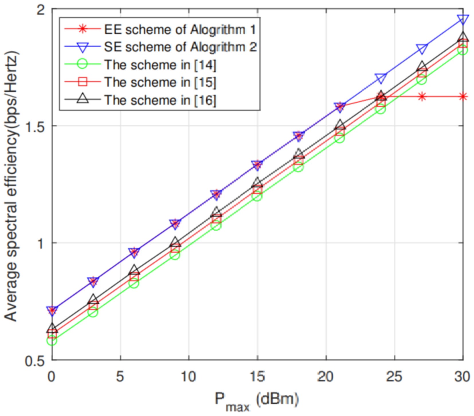
Figure 3.
Different resource allocation algorithms based on SE.
Table 2. Energy-efficient inner resource allocation algorithm, solving the optimization problem F(ηn−1).
1. Initialize: Set the maximum number of outer loop iterations Mmax, the dual variables $ \mu $ and $ \lambda $, set the outer loop iteration factor m = 0. 2. Outer Loop: 3. Initialize the maximum number of inner loop iterations Nmax and $ {\tau _I} $, and set the inner loop iteration factor n = 0; 4. According to Eq. (37) and ε(i, j), and using the golden section method, calculate A(i, j); 5. Inner Loop: 6. Calculate ϕ(i, j) according to Eq. (46) and Hungarian algorithm; 7. Update $ {\tau _I} $ according to Eqs (44), (45); 8. Through n = n + 1, update the inner loop iteration factor n; 9. End condition of inner loop: Inner loop convergence or n = Nmax. 10. According to Eq. (46), $ {\tau _I} $ and A(i,j) calculate P(i,j); 11. Use the sub-gradient method to update $ \mu $ and $ \lambda $, $ {\tau _I} $,P(i,j) and A(i,j); 12. Through m = m + 1, update the outer loop iteration factor m; 13. End condition of outer loop: Outer loop convergence or m = Mmax. 14. Calculate $ P_i^{S1} $, $ P_{i,j}^{S2} $ and $ P_{i,j,k}^R $ according to Eq. (18) and Eqs (40), (41). 15. Calculate Pi,j using Eqs (31)−(33). 16. Output $ \Phi $ and P. The performance of the SE optimal joint optimization Algorithm 2 proposed is significantly better than the previously published algorithms[14−16]. Not only because Algorithm 2 jointly optimizes sub-carrier pairing, power allocation, and EH time assignment, it also improves HTC to optimize SE performance. It can be seen from Fig. 3 that the performance curve of the proposed EE scheme of Algorithm 1 is different. Because the algorithm proposed can improve spectral efficiency on the premise of ensuring effective energy consumption. When PT > 21 dBm, the curve of spectral efficiency shows an upward trend. When PT ≤ 21 dBm, the curve tends to be stable. It is not difficult to find that power allocation is a very common resource allocation scheme. However, under the premise of not increasing the computational complexity, equal power allocation is a better strategy. Because the performance gain brought by the optimal power allocation algorithm is not significant.
In addition, the proposed Algorithm 2 at PT ≤ 21 dBm has higher SE performance than the algorithms previously published[14−16], and can achieve performance gains of approximately 0.39, 0.30, and 0.23 dB, respectively.
Figure 4 depicts the SE convergence performance curves at different maximum transmit powers PT. As shown in the figure, the SE performance gradually decreases after the start of the iteration, and tends to converge after the number of iterations exceeds seven. The larger the PT, the greater the SE performance can be obtained, but it does not affect the convergence performance of the iterative algorithm.
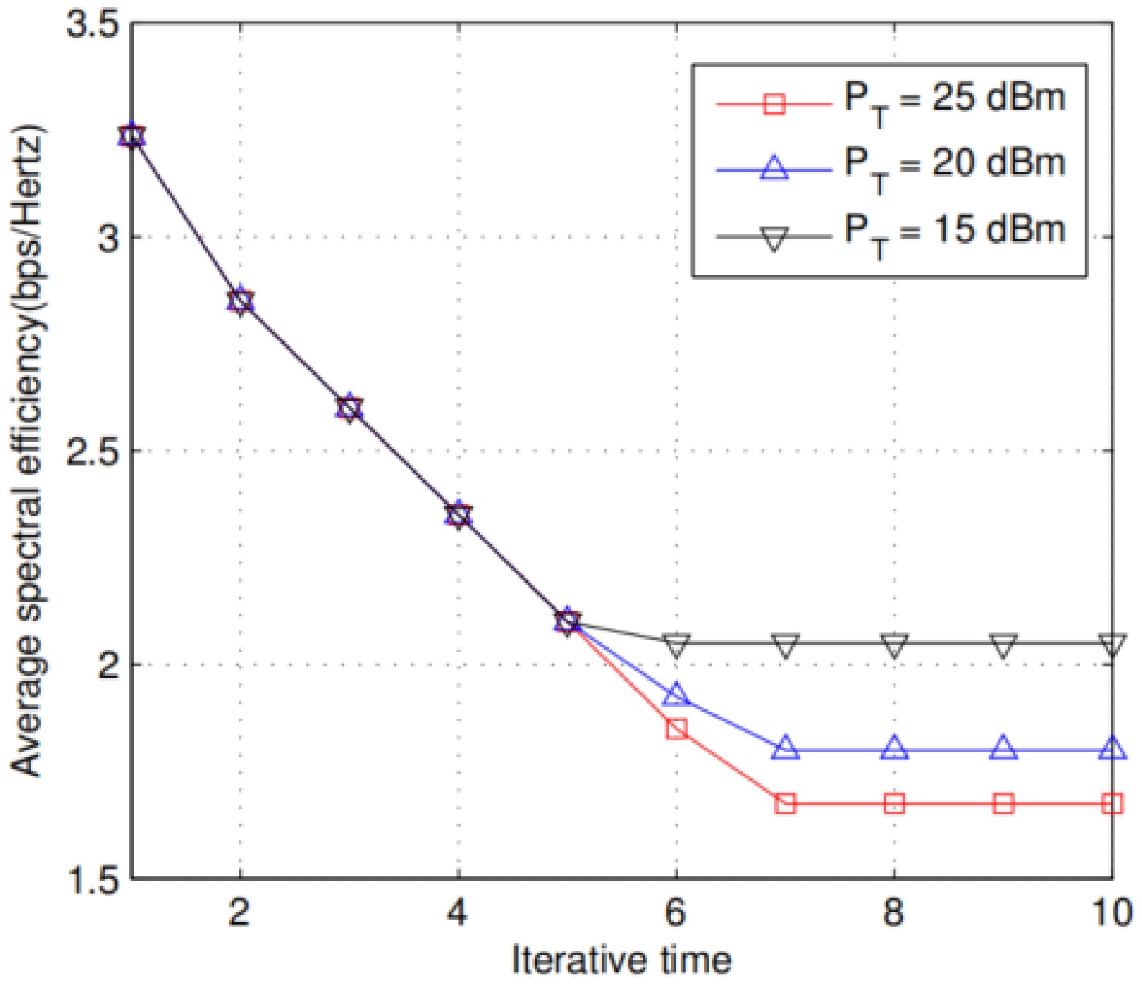
Figure 4.
The SE convergence of the proposed algorithm.
In Fig. 5, we compare the SE and EE performance of the proposed algorithm[14−16]. Because the optimization goal of Algorithm 2 and algorithms from previous studies[14−16] is to maximize SE. When PT ≤ 21 dBm, the EE curve increases monotonously, and when PT > 21 dBm it decreases monotonously. However, the proposed EE scheme of Algorithm 1 in this paper pursues the EE maximization. The EE performance curve grows rapidly when PT ≤ 21 dBm. However, when it grows close to the threshold point PT > 21 dBm, the curve growth slows down until it stabilizes and no longer changes. Because we design an optimal resource allocation scheme based on EE, the iteration stops once the EE performance of the system reaches the optimum. Even if it is possible to expend more energy for SE buffs, it will not take action. This strategy is shown in Fig. 5 where once the transmitted energy power exceeds the PT > 21 dBm, the EE performance does not change. This 21 dBm is the transmission power to be consumed to obtain the optimal EE, and it can be known that the optimal EE is 1.3 bit/J/ Hz through calculation. From Figs 3 and 5, due to the use of joint sub-carrier pairing, power allocation and EH time assignment and an improved HTC protocol, when PT ≤ 21 dBm, the proposed EE scheme of Algorithm 1 will gain better EE and SE performance than the algorithms previously published[14−16]. As can be seen from Fig. 5, the computational complexity of the above algorithms is not very different, but there is still a certain gap in performance. This confirms the importance of joint resource allocation from another perspective.
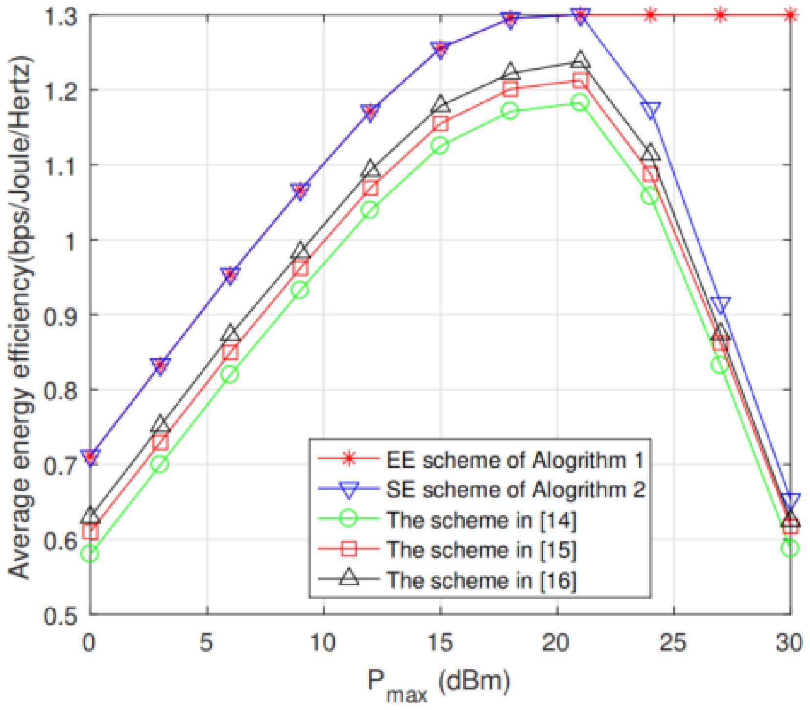
Figure 5.
Comparison of EE performance of different resource allocation algorithms.
Figure 6 depicts the convergence performance curves of EE at different maximum transmit powers PT. The EE performance gradually increases until saturation after the iteration starts. The iterative algorithm tends to converge after seven iterations. Consistent with the performance of Fig. 4, the larger the PT, the greater the EE performance can be obtained, but it does not affect the convergence performance of the iterative algorithm.
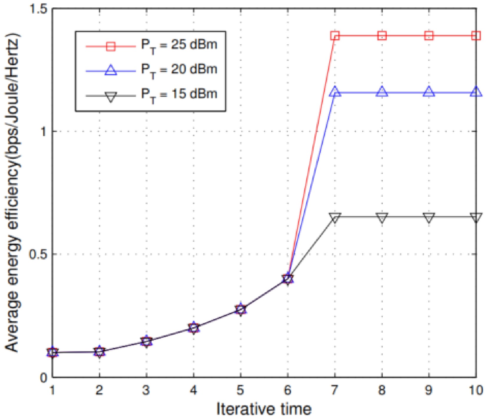
Figure 6.
The energy efficiency convergence of the proposed algorithm.
-
This paper proposes a joint resource allocation algorithm in energy harvesting scenarios. A three-phase energy harvesting collaborative communication protocol has been proposed to achieve greater diversity gain in the system. Then, a joint resource allocation model based on optimal energy efficiency was established. To solve this NP hard problem, a joint resource allocation algorithm based on optimal energy efficiency was proposed using the Dinkelbach method and the Cauchy inequality method. The simulation verified the low complexity and convergence of the algorithm. In future research, we can focus on the application of energy harvesting technology in the latest scenarios such as the Internet of Things and drones.
This study was supported by the Outstanding Young Backbone Teachers Program of "Qinglan Project" in Jiangsu Higher Education Institutions, the University-level Science and Technology Innovation Team Project of Nanjing Railway Vocational and Technical College (CXTD2023002), the Major Project of Basic Science (Natural Science) Research in Jiangsu Higher Education Institutions (23KJA520004), the General Projects of Philosophy and Social Sciences Research in Jiangsu Higher Education Institutions (2023SJYB0768, 2024SJYB0346), the Action Plan of the National Engineering Research Center for Cybersecurity Level Protection and Security Technology (KJ-24-004), and the Research Project on Degree and Postgraduate Education and Teaching Reform of Jiangsu Province (JGKT24_B036).
-
The authors confirm their contributions to the paper as follows: data collection: Xin J, Liang G; analysis and interpretation of results: Li L, Feng Y; draft manuscript preparation: Ni X, Xia L. All authors reviewed the results and approved the final version of the manuscript.
-
Data will be made available upon request from the corresponding author.
-
The authors declare that they have no conflict of interest.
- Copyright: © 2026 by the author(s). Published by Maximum Academic Press, Fayetteville, GA. This article is an open access article distributed under Creative Commons Attribution License (CC BY 4.0), visit https://creativecommons.org/licenses/by/4.0/.
-
About this article
Cite this article
Xin J, Liang G, Li L, Ni X, Xia L, et al. 2026. Energy efficiency resource allocation for amplify and forward relaying system with energy harvesting. Wireless Power Transfer 13: e004 doi: 10.48130/wpt-0025-0021 

Energy efficiency resource allocation for amplify and forward relaying system with energy harvesting
- Received: 27 August 2024
- Revised: 22 October 2024
- Accepted: 05 November 2024
- Published online: 02 February 2026
Abstract: With the vigorous advocacy of green communication, research on energy harvesting technology in mobile communication resource allocation has become increasingly urgent. This paper studies the resource allocation problem of multi-relay energy harvesting systems. To improve the diversity gain of the relay system, an improved three-phase energy harvesting relay protocol is proposed. Complete with established non-convex optimization models and transform them into quasi-convex problems through convex optimization methods. Then, by constructing a nonlinear programming model with optimal energy efficiency, parameters such as energy harvesting time slot allocation, subcarrier pairing, and power allocation are jointly optimized. Finally, the Dinkelbach method and Hungarian algorithm were used to iteratively obtain the optimal solution. The Monte Carlo simulation experiment verified the accuracy and fast convergence of the algorithm.
-
Key words:
- Energy /
- Efficiency /
- Resources /
- Relaying /
- RF