-

Figure 1.
(a) Soil RubisCO activity and (b) cbbL gene abundances in different treatments. Values are means (n = 3), and error bars represent standard deviation. Different lowercase letters above columns indicate significant differences (one-way ANOVA, P < 0.05) among treatments.
-
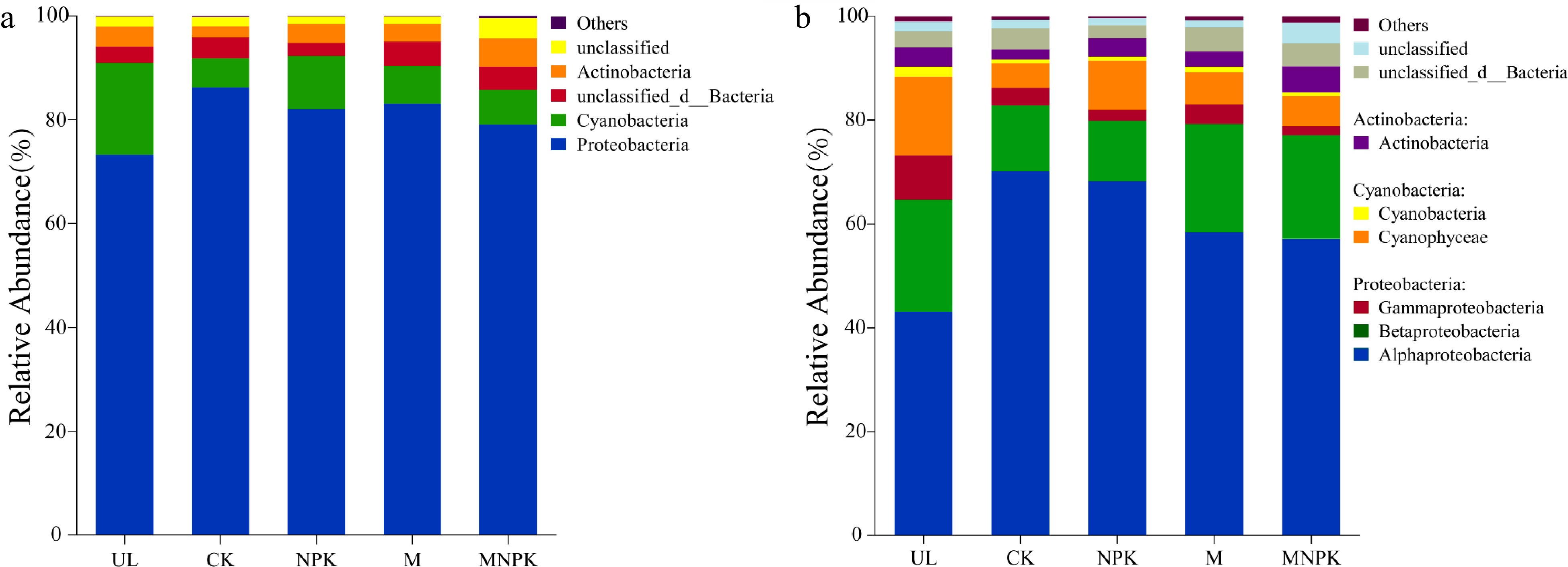
Figure 2.
Taxonomic composition of carbon-fixing microbial communities in soils at (a) phylum level and (b) class level.
-
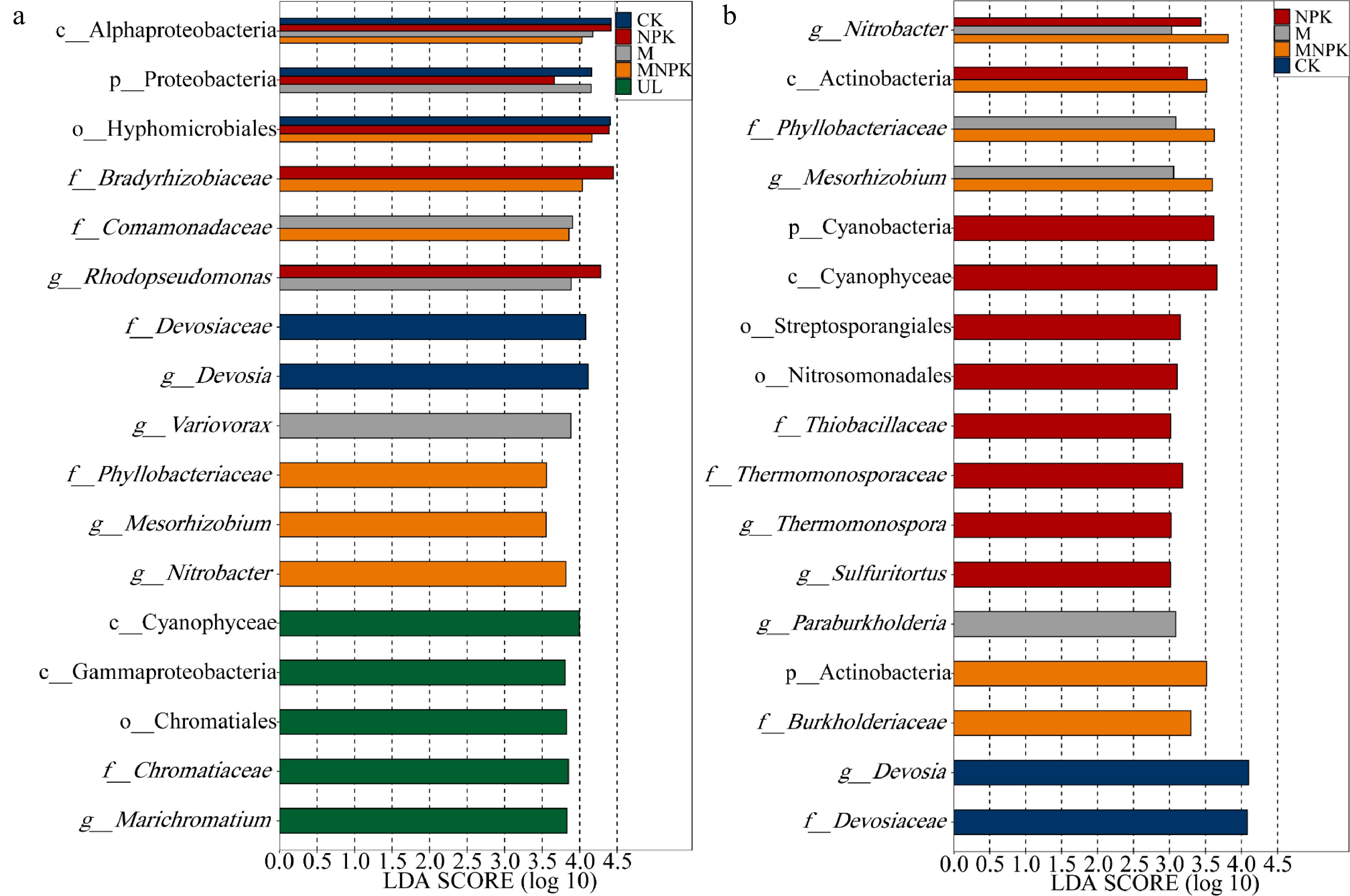
Figure 3.
Linear discriminant analysis (LDA) effect size analysis determined biomarkers (a) between UL and other treatments (CK, NPK, M and MNPK) and (b) between CK and fertilization treatments (NPK, M and MNPK). The LDA score indicates the effect size and ranking of each differentially abundant taxon (P < 0.05, LDA score > 3.5, a) (P < 0.05, LDA score > 3.0, b). The ordinate is the taxon with significant difference among groups, and the abscissa is a bar chart to visually show the LDA log score of each taxon. Blue, red, gray and orange bars represent the biomarkers in CK, NPK, M and MNPK having significantly greater abundances than in UL, respectively (a). Green bars represent the biomarkers in UL having significantly greater abundances than in all the other four treatments (a). Gray orange and red bars represent the biomarkers in M MNPK and NPK having significantly greater abundances than in CK, respectively (b). Blue bars represent the biomarkers in CK having significantly greater abundances than in all the other three treatments (b).
-
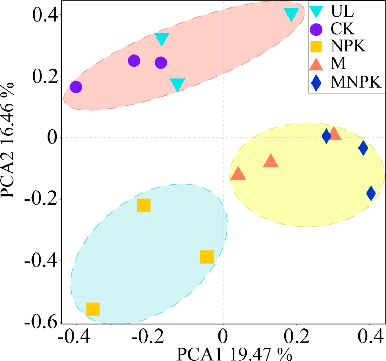
Figure 4.
Principal component analysis (PCA) of the carbon-fixing microbial community in different treatments.
-
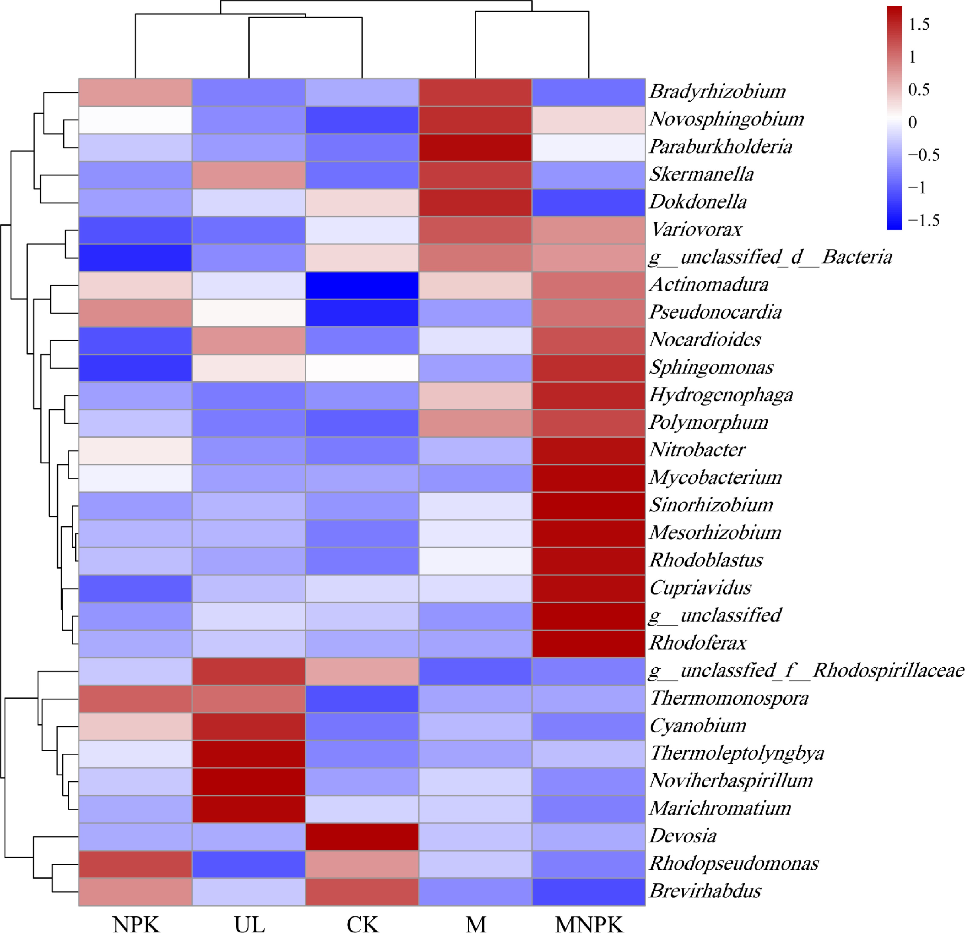
Figure 5.
Biclustering heatmap of the carbon-fixing microbial distributions of the top 30 abundant genera is present in different treatments. The color intensity of the color lumps represents the abundance of the carbon-fixing microbial genera in different treatments, with red representing higher abundance and blue representing lower abundance.
-
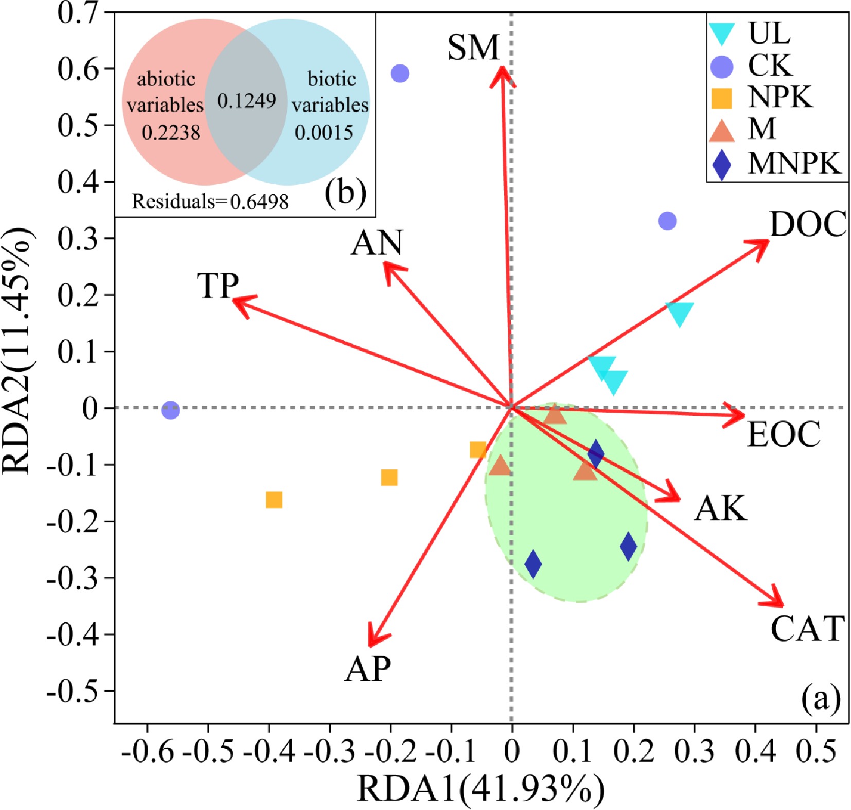
Figure 6.
(a) Redundancy analysis (RDA) linking carbon-fixing microbial communities with environmental variables in different treatments. Arrows represent the correlation between the soil properties and carbon-fixing microbial communities. Variables that are angled at more than 90° of each other have the least correlation. The length of the arrow represents the correlation. Variables that have arrows extended in opposite directions correlate negatively to each other. (b) Diagrams explaining variance partitioning (VPA) show the relative contribution of ecological drivers with VIF < 5 to soil carbon-fixing microbial community structure. The abiotic variables include EOC, AP, DOC, AK, SM, TP and AN; the biotic variables include CAT. The numbers are the percentages of the total variables explained by the factors.
-
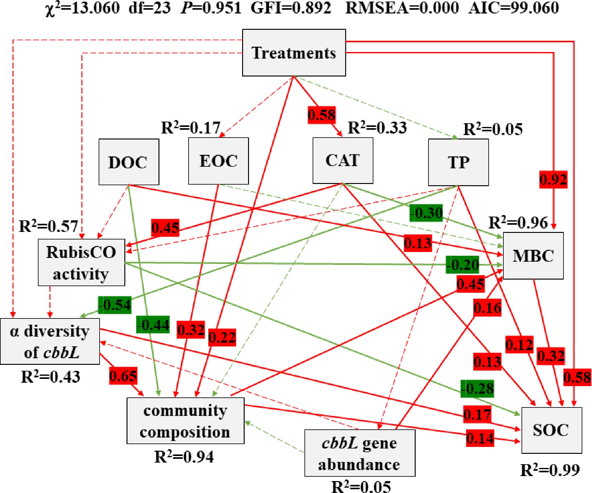
Figure 7.
Structural equation model (SEM) shows the causal influences of treatments, DOC, EOC, CAT, TP, RubisCO activity, α diversity of cbbL, community composition (carbon-fixing microbial community), cbbL gene abundance, SOC and MBC. Positive and negative effects are respectively showed in red and green, and significant and non-significant effects are showed with solid and dashed arrow lines, respectively. The standardized coefficients are marked above each path (only marked significant effect paths) and indicate the expected impact of a unit standard-deviation change at one node on units of standard-deviation change in connected nodes. R2 values represent the proportion of the variance explained for each endogenous variable.
-
Index Treatments UL CK NPK M MNPK SM (g·kg−1) 0.17 ± 0.02ab 0.19 ± 0.02a 0.15 ± 0.01b 0.18 ± 0.01ab 0.15 ± 0.01b pH 8.27 ± 0.09a 7.86 ± 0.49a 7.85 ± 0.42a 8.15 ± 0.06a 8.14 ± 0.13a TN (g·kg−1) 0.27 ± 0.04c 0.32 ± 0.06bc 0.40 ± 0.07b 0.56 ± 0.01a 0.59 ± 0.06a AN (mg·kg−1) 304.05 ± 0.00ab 344.59 ± 11.50a 302.85 ± 30.84ab 315.97 ± 145.67ab 174.08 ± 99.02b TP (g·kg−1) 0.38 ± 0.00a 0.69 ± 0.46a 0.39 ± 0.20a 0.35 ± 0.28a 0.39 ± 0.20a AP (mg·kg−1) 5.09 ± 0.00b 10.93 ± 0.26ab 17.68 ± 5.80a 12.14 ± 0.80ab 18.65 ± 7.16a TK (g·kg−1) 5.61 ± 0.00a 3.72 ± 0.74b 2.88 ± 1.40b 3.20 ± 0.03b 4.01 ± 0.70b AK (mg·kg−1) 80.06 ± 0.00a 74.71 ± 8.34a 77.39 ± 8.34a 86.73 ± 10.08a 86.74 ± 15.17a CAT (ml·g−1) 2.15 ± 0.06a 1.52 ± 0.22b 1.65 ± 0.03b 2.22 ± 0.05a 1.97 ± 0.26a SOC (g·kg−1) 1.74 ± 0.00c 1.55 ± 0.08c 2.07 ± 0.17b 3.35 ± 0.24a 3.12 ± 0.04a MBC (mg·kg−1) 9.85 ± 0.45d 17.06 ± 1.50c 19.72 ± 0.58b 37.78 ± 2.29a 37.45 ± 0.82a DOC (g·kg−1) 0.09 ± 0.01a 0.09 ± 0.02a 0.08 ± 0.01a 0.08 ± 0.01a 0.08 ± 0.01a POC (g·kg−1) 0.24 ± 0.23a 0.28 ± 0.15a 0.52 ± 0.12a 0.60 ± 0.18a 0.71 ± 0.57a EOC (g·kg−1) 1.58 ± 0.22a 1.48 ± 0.58a 1.34 ± 0.35a 1.93 ± 0.46a 1.65 ± 0.69a Values indicate mean ± standard deviations (n = 3). Different letters in each row represent a significant difference among treatments (one-way ANOVA, P < 0.05). Table 1.
Soil biophysicochemical properties in different treatments
Figures
(7)
Tables
(1)