Road traffic intensity of GDP and the explanation of national peaks of yearly road fatalities and of their clustering in 1970−1974

Marc Gaudry; Lasse Fridstrøm; Marc Gaudry; Lasse Fridstrøm

doi:10.48130/EMST-2023-0006

Figures (13) Tables (10)

Figure 1.
Effect of three speed limit changes on the frequency of fatal accidents on French highways^[39,54].
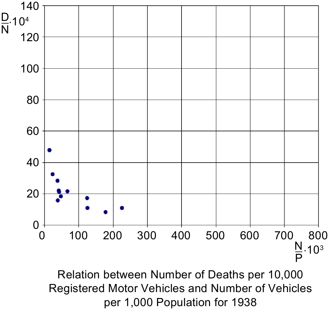
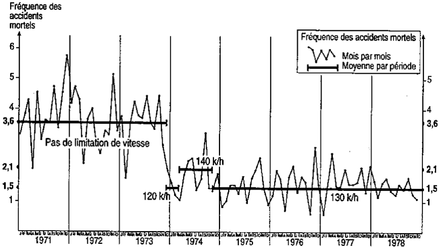
Figure 2.
Fatalities per vehicle and vehicles per capita (Smeed's 1938 data in S-5 sample).
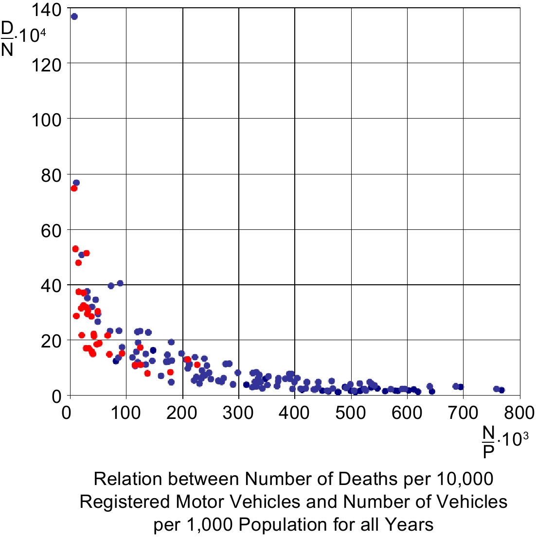
Figure 3.
Fatalities per vehicle and vehicles per capita (Smeed‘s 1931; S-5 and S-6 samples).
Figure 4.
Fatalities per 10,000 vehicles and vehicles per 1,000 inhabitants over time in 26 countries.
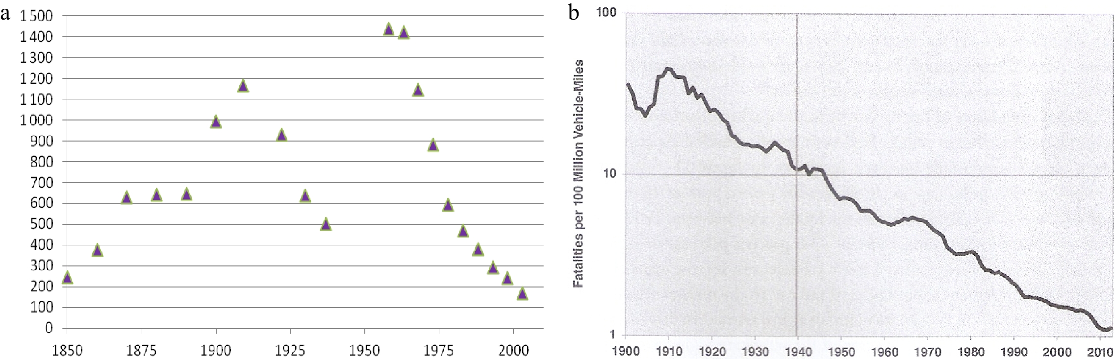
Figure 5.
Secular fatality intensity of road traffic in France (1845−2005) and the USA (1900−2012). (a) Index of the fatality intensity of total road traffic. Deaths caused by horses, horse-drawn carriages and automobiles in France, 1845−2005 (mostly quintannual) (Source: ^[45], Figure 4.F, p. 14). (b) Logarithm of motor vehicle road deaths per 100 million vehicle-miles in the USA, 1900−2012 (yearly) (Source: ^[46], Figure 11-6, p. 386).
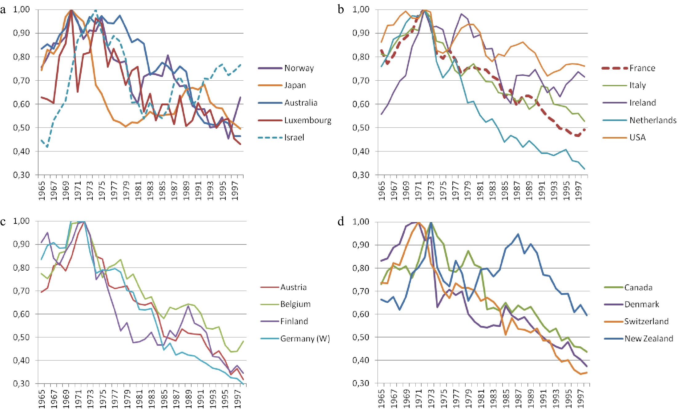
Figure 6.
Meadow-shaped evolutions of yearly road fatalities in the 18 OCDE lustrum countries. (a) Fatality indices, 1965−1998: Norway, Japan, Australia, Luxemburg (1970 = 1.00), Israel (1974 = 1.00). (b) Fatality indices, 1965−1998: France, Italy, Ireland, Netherlands, USA (1972 = 1.00). (c) Fatality indices, 1965−1998: Austria, Belgium, Finland, West Germany (1972 = 1.00). (d) Fatality indices, 1965−1998: Denmark & Switzerland (1971 = 1.00), Canada & New Zealand (1973 = 1.00). Source: Gaudry^[51], except the series for Israel from www.cbs.gov.il/publications16/acci15_1643/pdf/gr01_e.pdf.
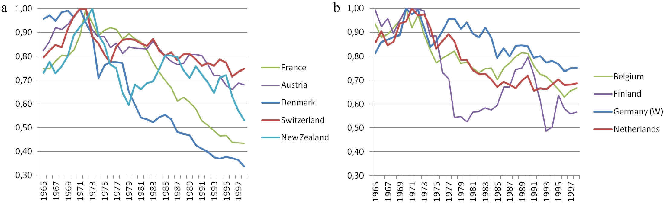
Figure 7.
Lustrum country injury peaks simultaneous to, or preceding, their own fatality peaks. (a) Injury peaks synchronized with death peaks, 1965−1998: Denmark, Switzerland (1971 = 1.00); France, Austria (1972 = 1.00); New Zealand (1973 = 1.00). (b) Injury peaks occurring earlier than 1972 death peaks, 1965−1998: Belgium, Finland, West Germany (1970 = 1.00); Netherlands (1971 = 1.00). Source: all series are from the MAYNARD-DRAG database^[50].
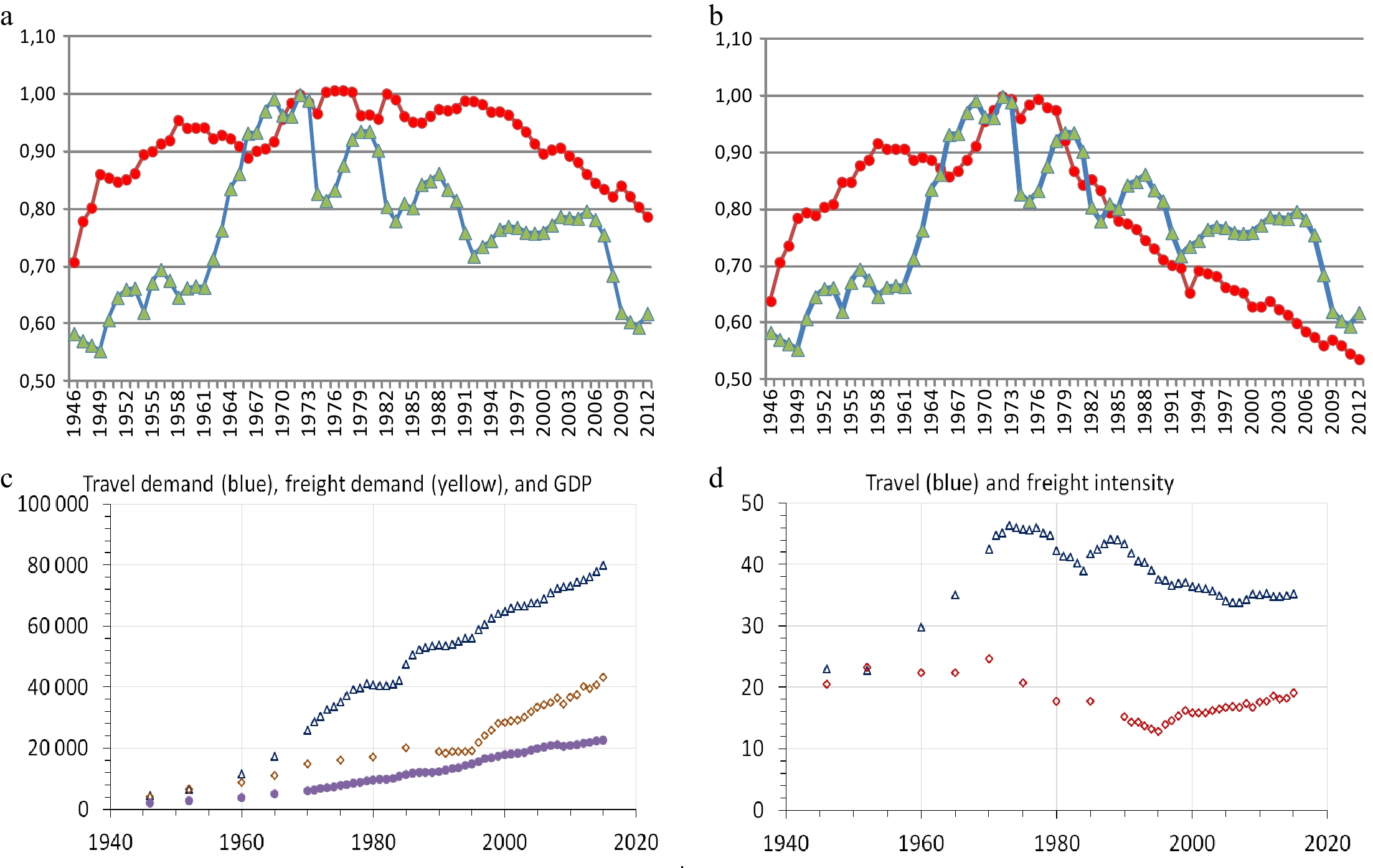
Figure 8.
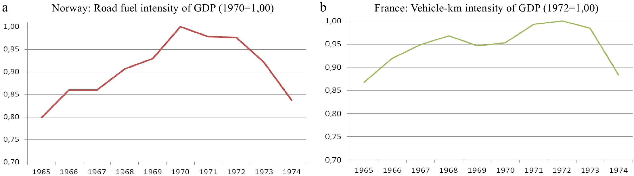
Measures of national transport intensity of GDP (in constant national currencies). Upper pannel, Fatality (1972 = 1) and Road traffic intensity of GDP indices (1972 = 1) for the USA, 1946−2012. (a) [Fatalities () and] Mile intensity of GDP (). (b) [Fatalities () and] Gallon intensity of GDP (). Lower pannel, Norwegian GDP and all-mode transport intensities, 1946, 1952, 1960, 1965 and 1970−2015. (c) Domestic travel-km & freight-km and GDP in Norway. (d) Travel & freight transport intensities of GDP in Norway. Sources: ^[69] for the Mile and Gallon intensities of GDP (); NHTSA Safety Facts (Various years) for Fatalities (). Lower pannel source: Lasse Fridstrøm. Produced on 22^nd October, 2017.
Figure 9.
Road fuel and Vehicle-km indices of road use intensity of GDP (defined over 1965−1998). Source: all series are extracted or derived from the MAYNARD-DRAG database^[41] except for the GDP series for France, which is from INSEE. The traffic intensity indices are defined over the period 1965−1998.
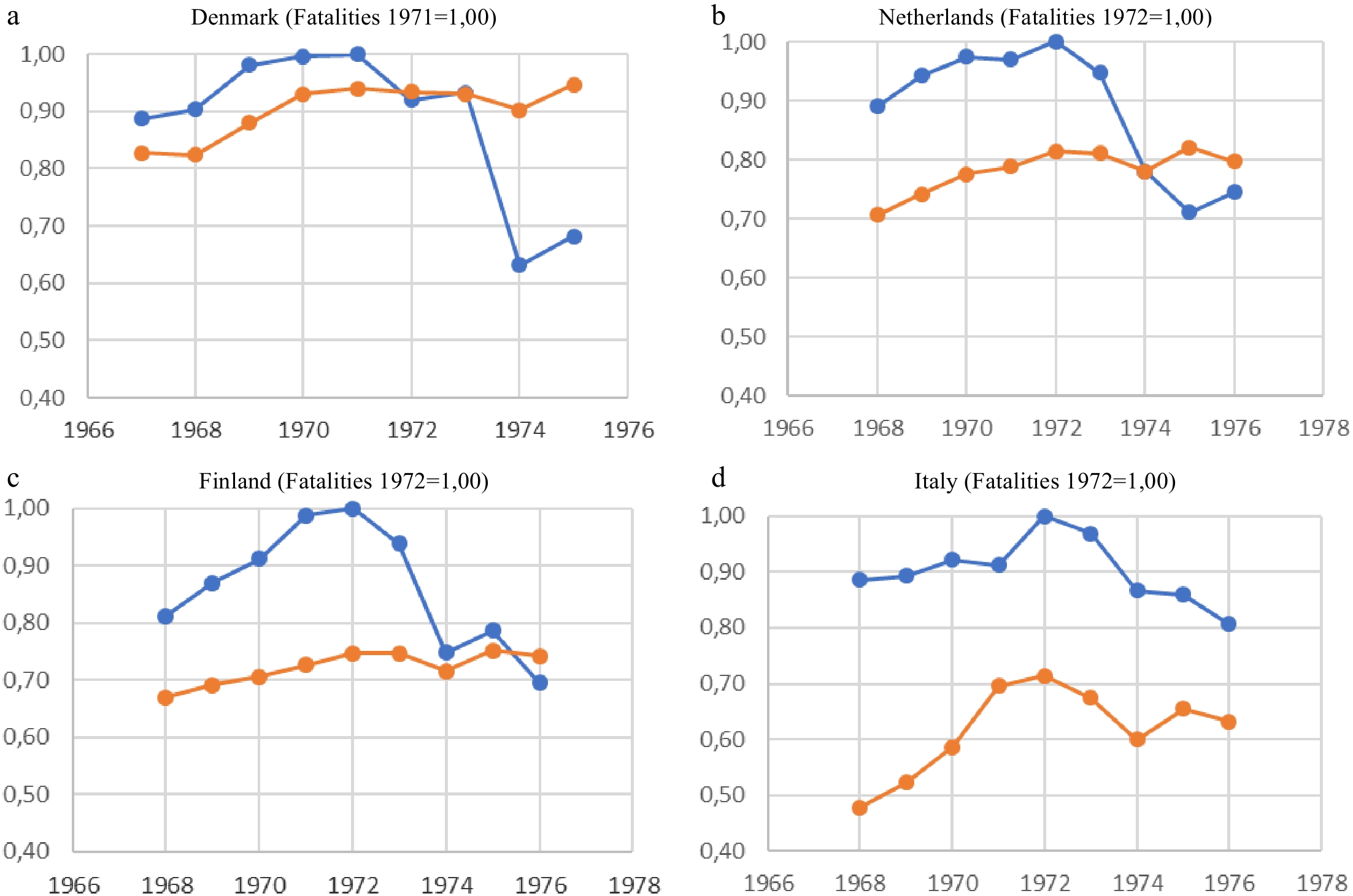
Figure 10.
Global maxima of fatalities (at 1.00) and local maxima of road traffic intensities of GDP.
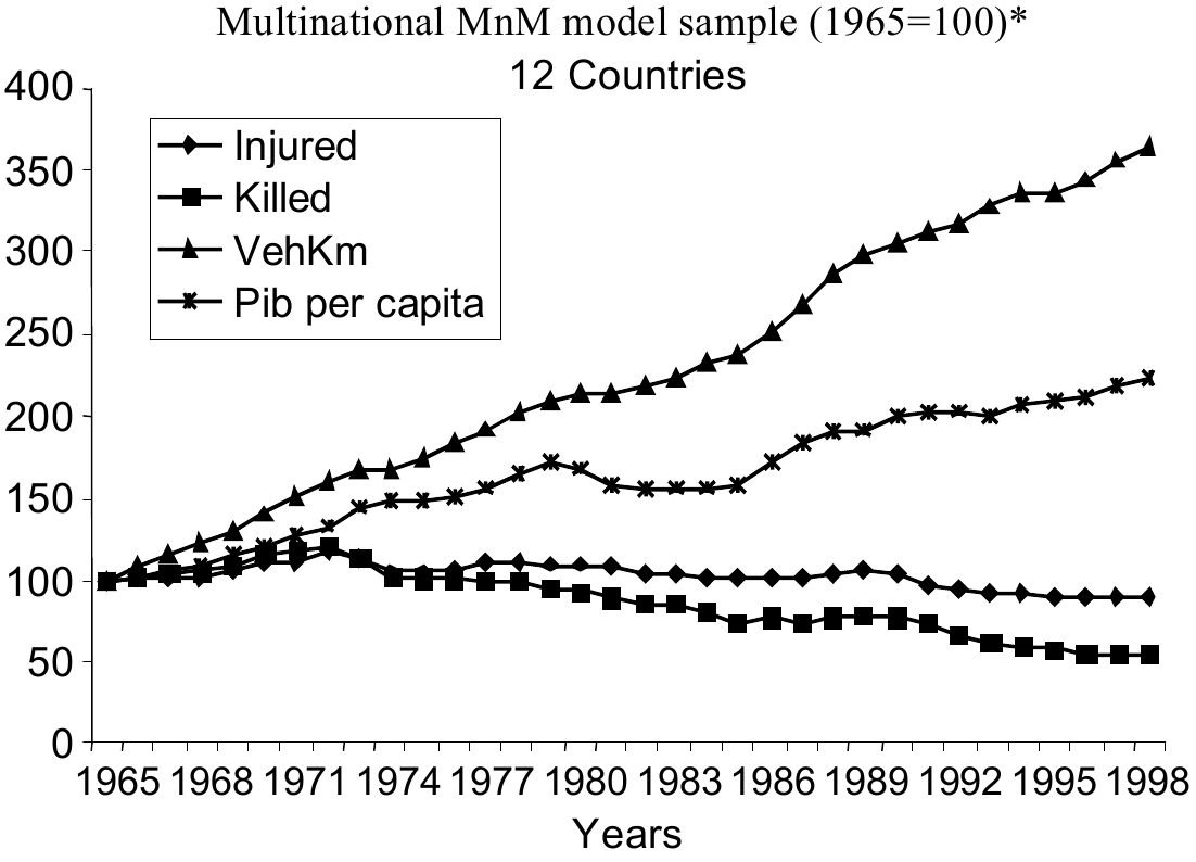
Figure 11.
Indices of road use, GDP per capita, and killed or injured victims in our sample. * The 12 OECD countries selected in Table 4 (1965−1998 data).
Figure 12.
Ratio of initial to enriched residuals wt during the five lustrum Matterhorn years 1970−1974. (a) Accident equation, 65 observations for the Matterhorn period, 13 regions per year for 5 years (1970−1974)*. (b) Injured equation, 65 observations for the Matterhorn period, 13 regions per year for 5 years (1970−1974)**. (c) Killed equation, 65 observations for the Matterhorn period, 13 regions per year for 5 years (1970−1974)***. [* The average ratio of initial to enriched Accident errors values for the full estimation sample period (1967−1999) is 0.96. ** The average ratio of initial to enriched Injured errors values for the full estimation sample period (1967−1999) is 1.14. *** The average ratio of initial to enriched Killed errors values for the full estimation sample period (1967−1999) is 0.32.]
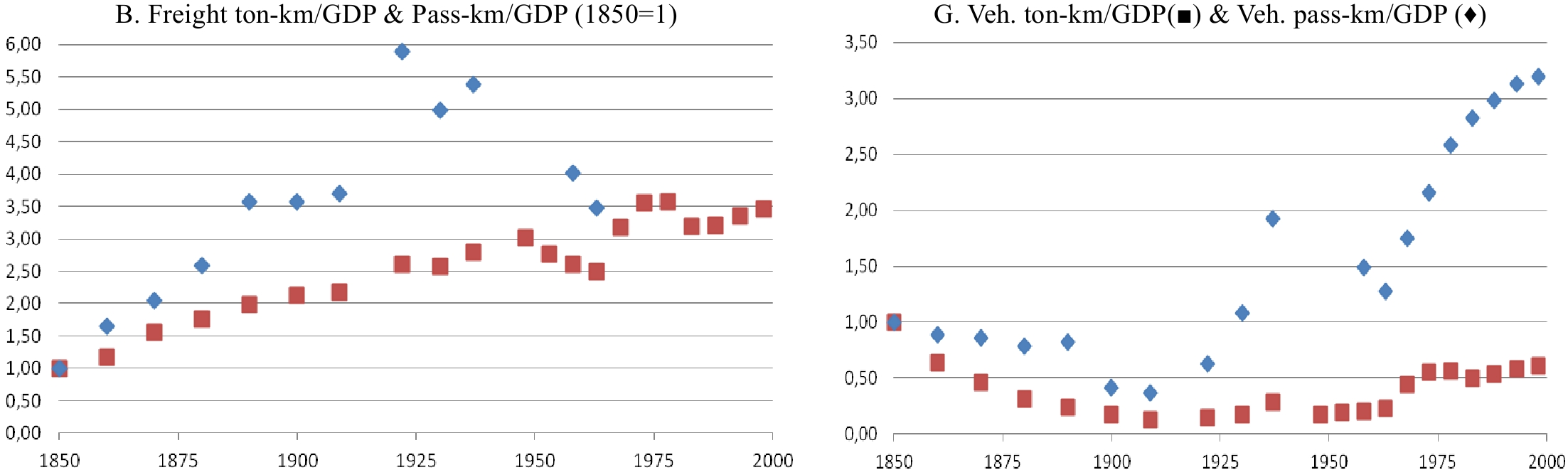
Figure 13.
Road flow and vehicle intensities of GDP (ton-km & pass-km), France 1845−2005. Source: Gaudry^[24] (Fig. 2, p. 6), where the transformation from flows in B to vehicles in G is described in detail.

Demand for road use (DR) by gasoline and diesel vehicles				Crash frequency (A) & severity (G)
Gasoline road use demand: elasticity of veh-km with respect to		Diesel road use demand: elasticity of veh-km with respect to		Effect of DR and trip purpose demand mix, i.e. of each (activity level/DR), on A or G
Work	0.40	Manufacturing: deliveries	0.80	Work/DR	Yes
Shopping	0.24			Shopping/DR	Yes
Vacation and summer fairs	0.05			Vacation/DR	Yes
Home deliveries	0.05	Home deliveries	0.04
		Forestry output	0.14	Forestry output/DR	Yes
Residential construction input	0.02	Large dam construction inputs	0.03	Residential construction input/DR	Yes
		Engineering works: deliveries	0.02
Agricultural output	0.05	Agricultural output	0.02	DR	Yes
Sum of gasoline elasticities evaluated at sample means:	0.81	Sum of diesel elasticities evaluated at sample means:	1.05	Each such trip purpose ratio indicator is significant relatively to reference (other).
Source: Appendix 1. Detailed Model Outputs, § 1.2, Fournier & Simard^[29]. Ch. 15, p. 347, Gaudry & Lassarre^[30].

Table 1.

Recurrent intermediate and/or final activities present in the DRAG-2 model (1956−1993).

Smeed’s original equation					Years	n. obs.	R²
S-1	(Killed/Vehicles) =	k (Vehicles/Population)^–2/3
S-2	(Killed) =	k (Vehicles)^1/3 / (Population)^2/3
S-3	(Killed) =	k (Vehicles)^1/3 / (Population)^2/3
S-4	Ln (Killed) =	Ln (k) + 0,333 Ln (Vehicles) + 0,667 Ln (Population)			1938	20
Our estimates with Smeed’s own equation with more recent data
S-5	Ln (Killed) =	Ln (k) + 0,408 Ln (Vehicles) + 0,699 Ln (Population) (16,31) (20,41)			1938* to 1946	210	0,98
S-6	Ln (Killed) =	Ln (k) – 0,058 Ln (Vehicles) + 1,100 Ln (Population) (-3,36) (55,92)			1965 to 1998	918	0,88
Note 1. Ln denotes natural logarithm and (t-statistics) are provided in parentheses. Note 2. Sample S-5 is from Smeed (1949) and sample S-6 is from MAYNARD-DRAG.
* The 17 countries for 1938 in sample S-5 are:	Portugal	Finland	South Africa	Canada	Australia	USA
	Ireland	Norway	New Zealand	Italy	Netherlands	France
	Northern Ireland	Sweden	Denmark	Great Britain	Switzerland

Table 2.

Smeed's original country set data base, specification and results with various samples.

P	Price		Minimum gasoline price
M	Motorization		Proportion of cars in total vehicle fleet
	Congestion		Percentage of urban population in total population
N	Network	Legal	Highway speed limit (km/h)
			Seatbelt regulation (dummy)
		Climate	Temperature (yearly average)
			Total yearly precipitation (mm)
Y	Driver	Age	Percentage of 18-24 years old in total population
			Percentage of 65 years old or older in total population
A	Final economic output		GDP per capita
	Total/Final economic output		Road traffic intensity of GDP (Vehicle-km/GDP) index I
ETC.			Leap year, Dummy by region relative to that of reference region r

Table 3.

Regressors in MnM-2 model of accident frequency, their severity and victims by category.

Appendix 2 values:	Fatalities per 10,000 inhabitants			Injuries per 10,000 inhabitants
13 regions included in MnM model sample	In 1998 (Rank 1-26)	% change 1972−1998	Speed rank (1−26)	In 1998 Unranked	% change 1972−1998	Speed rank (1−26)
Australia	0.940 (10)	−63.795	7	11.114	−83.686	1
1. Austria	1.192 (15)	−70.423	3	63.230	−36.737	8
2. Belgium	1.470 (21)	−53.975	14	69.345	−34.893	9
11. Canada	0.966 (11)	−65.849	6	71.503	−27.094	12
3. Denmark	0.856 (9)	−61.690	8	16.767	−66.208	2
Finland	0.776 (4)	−68.843	4	17.654	−48.756	6
4. France	1.515 (23)	−56.743	11	28.640	−61.874	3
Germany (East)	1.417 (20)	0.755	25	63.181	123.166	25
5. Germany (West)	0.842 (7)	−72.476	1	60.013	−30.165	11
6. Great Britain (UK)	0.594 (1)	−58.237	10	55.917	−13.355	13
Greece	2.117 (25)	64.779	26	31.780	10.670	21
Hungary	1.356 (19)	−22.071	21	26.095	0.974	19
Iceland	0.985 (12)	−10.457	23	51.022	−10.765	15
Ireland	1.236 (16)	−41.591	17	34.475	16.418	22
Italy	1.098 (14)	−50.070	15	51.024	3.622	20
Japan	0.855 ( 8)	−55.724	13	78.244	−5.681	17
Luxembourg	1.336 (18)	−56.519	12	36.545	−51.246	5
7. Netherlands	0.679 (3)	−72.269	2	31.560	−39.975	7
New Zealand	1.324 (17)	−46.121	16	32.730	−57.435	4
8. Norway	0.794 (5)	−36.251	19	27.347	−4.954	18
Portugal	2.133 (26)	−16.477	22	69.163	73.759	24
13.Quebec	(0.987) (12−13)	(−69.774)	(3−4)	(64.194)	(−22.418)	(12−13)
12.Spain	1.513 (22)	−9.965	24	35.909	30.490	23
9. Sweden	0.600 (2)	−59.194	9	24.126	−7.813	16
10.Switzerland	0.840 (6)	−67.879	5	39.108	−32.709	10
Turkey	1.011 (13)	−26.192	20	18.201	223.304	26
USA	1.534 (24)	−41.007	18	118.091	−11.304	14
Portugal / Great Britain	3.6 ≡ Max / Min		26/1	1.2		24/13
USA / Australia	1.6		18/7	10.6 ≡ Max / Min		26/1
	(1.06; 1.15) ≡ (Median; Mean) of 26			36.23; 44.72 ≡ (Median; Mean) of 26
Source: all series are from the MAYNARD-DRAG database^[50].

Table 4.

Evolution of per capita fatalities and injuries in 26 countries and Quebec, 1972−1998.

Year	n	The 26 countries of Appendix 1 (plus Israel, minus Turkey)*
1965−1966	2	Great Britain, Sweden
1970	4	Australia, Luxemburg, Norway, Japan
1971	2	Denmark, Switzerland
1972	9	Austria, Belgium, France, Finland, Germany (W), Ireland, Italy, Netherlands, USA
1973	2	Canada, New Zealand
1974	1	Israel
1975	1	Portugal
1977	(1/2)	Germany (E) before reunification
1988	1	Iceland
1989	1	Spain
1990	1	Hungary,
1991	(1/2)	Germany (E) after reunification
1998	1	Greece
* Note: to define a global national maximum, WWII years are excluded for Great Britain which really peaked in 1940−1941.

Table 5.

Year of the global maximum of road fatalities in 26 countries, 1965-1998.

CASE		${\beta _{Q1}}$	$ {\beta _{Q2}} $	${\lambda _{Q1}} - {\lambda _{Q2}}$	$ {\beta _{Q1}}({\lambda _{Q1}} - {\lambda _{Q2}})$ or $ {\beta _{Q2}}({\lambda _{Q2}} - {\lambda _{Q1}})$
∩	Maximum 1	+	−	−	−
$\cup $	Minimum 1	+	−	+	+
∩	Maximum 2	−	+	+	−
$\cup $	Minimum 2	−	+	−	+
Source: ^[⁶⁶^].

Table 6.

Sign conditions for a maximum or a minimum with two BCT on a repeated variable.

Year of maximum deaths (and fatality rate) and corresponding per capita GDP (1985 US dollars)
1965	Sweden	12,291	1972	Austria	13,219	1972	USA*	14,649
1966	UK	8,306		Belgium	13,271	1973	Canada	10,638
1970	Australia	9,988		Finland	12,107		New Zealand	10,591
	Luxembourg	15,550		France	13,434	1975	Portugal	4,715
	Japan	15,200		Germany (West)	11,581	1988	Iceland	19,752
	Norway	11,824		Italy	8,541	1989	Spain	9,825
1971	Denmark	16,579	1972	Ireland	6,001	1998	Greece	9,218
	Switzerland	28,670		Netherlands	13,356
MEAN: 16,526			STANDARD ERROR: 6,409			COEFFICIENT OF VARIATION: 0,39
* MAYNARD-DRAG database values in 1995 dollars have been adjusted by 0,761 from the US GDP deflator.

Table 7.

Actual per capita GDP of countries at the observed turning point of their road fatalities.

Column		1	2	3	4	5
I. Sample elasticity (conditional t-statistic)	Variant =	acc7	mbe7	mte7	ble7	tue7
	Version =	23	4	4	6	4
	DEP. VAR. =	Accidents Morbidity Mortality Injured Killed
P - Price
Minimum price per li of ordinary gazoline	PrixEss	−0.052	0.001	0.071	−0.087	−0.088
		(−2.98)	0.08	1.73	(−3.83)	(−2.81)
M - Motorization
Percentage of cars in the total of vehicles	PctAuto	0.114	−0.118	0.807	0.166	0.274
		−0.75	(−2.58)	3.66	1.00	1.34
Urban population (% of total population)	PctUrban	1.044	0.103	0.548	1.847	1.055
		(1.17)	(1.42)	(2.05)	(2.09)	(0.99)
N-L - Network-Regulations
Highway speed limit	HwySpeed	−0.023	−0.014	−0.241	−0.018	−0.069
		(−0.86)	(−0.57)	(−2.68)	(−0.63)	(−1.64)
SeatBelt regulations	SeatBelt	−0.029	0.000	−0.101	−0.036	−0.043
	===	(−2.19)	(0.00)	(−3.64)	(−2.85)	(−2.00)
Y - Socio-economic
Percentage of the population 65 and older	Pop65	0.192	−0.052	−0.661	0.240	0.529
		(0.62)	(−3.28)	(−6.71)	(0.63)	(1.09)
Proportion of the population 18-24 years old	PopYoung	0.305	−0.082	0.444	0.137	0.342
		(3.61)	(−7.35)	(5.97)	(0.96)	(1.84)
A - Economic activity
GDP per capita	PibCapit	0.310	−0.029	−0.421	0.478	0.501
		(3.78)	(−3.53)	(−8.70)	(4.61)	(3.83)
ETC.- Other Leap year	AnneeBis	0.002	−0.001	−0.001	−0.001	0.001
	===	(0.75)	(−0.31)	(−0.05)	(−0.31)	(0.11)
CS – Country-specific and Climate	See Appendix 4
Regression Constant	CONSTANT	−	−	−	−	−
		(0.44)	(1.54)	(0.16)	(−0.53)	(−0.97)
DELTA coefficient in Heteroskedasticity structure
Vehicle-Kilometer	VehKm	−0.000	−0.002			−0.019
		(−5.97)	(−10.96)			(−3.08)
II. Parameters
Heteroskedasticity Structure
BOX-COX Transformations: Unconditional [t-statistic = 0] and [t-statistic = 1]
LAMBDA(Z)	VehKm	7.469	−0.061			3.729
[t = 0]		[4.37]	[−0.27]			[2.23]
[t = 1]		[3.79]	[−4.75]			[1.63]
Autocorrelation
Order 1	RHO 1	0.953			0.967	0.974
		(86.09)			(75.98)	(116.80)
III. General Statistics
LOG-Likelihood		−3970.60	867.981	1624.209	−4146.47	−2794.25
PSEUDO-R2 :
- (E)		0.997	0.847	0.870	0.996	0.992
- (L)		0.999	0.885	0.916	0.999	0.999
- (E) Adjusted for D. F.		0.997	0.837	0.863	0.996	0.992
- (L) Adjusted for D. F.		0.999	0.878	0.911	0.999	0.998
Average Probability (Y = limit observation)		0.000	0.000	0.000	0.000	0.000
SAMPLE
- Number of observations		429	429	429	429	429
- First observation		27	27	27	27	27
- Last observation		455	455	455	455	455
Number of estimated parameters
- Fixed Part :
BETAS		24	24	24	24	24
BOX-COX		0	0	0	0	0
Associated dummies		0	0	0	0	0
- Autocorrelation		1	0	0	1	1
- Heteroskedasticity
Deltas		1	1	0	0	1
BOX-COX		1	1	0	0	1

Table 8.

Initial MnM-2 model for 12 countries and Quebec, 1965−1999, 455 observations.

Column		1	2	3	4	5
I. Sample elasticity (conditional t-statistic)	Variant =	acc7	mbe7	mte7	ble7	tue7
	Version =	22	3	3	5	3
	DEP. VAR. =	Accidents Morbidity Mortality Injured Killed
P - Price
Minimum price per li ordinary gasoline	PrixEss	−0.049	0.008	0.069	−0.073	−0.079
		(−2.58)	(1.02)	(1.65)	(−2.85)	(−2.46)
M - Motorization
Percentage of cars in PctAuto the total of vehicles	PctAuto	0.106	−0.069	0.805	0.122	0.112
		(0.74)	(−1.60)	(3.65)	(0.77)	(0.56)
Urban population (% of total population)	PctUrban	1.020	0.094	0.547	1.707	0.132
		(1.10)	(1.25)	(2.04)	(1.90)	(0.12)
N-L - Network-Regulations
Highway speed limit	HwySpeed	−0.009	0.009	−0.246	−0.002	−0.006
		(−0.33)	(0.37)	(−2.70)	(−0.07)	(−0.16)
SeatBelt regulations	SeatBelt	-0.027	-0.004	-0.100	-0.033	-0.039
	===	(−1.95)	(−0.92)	(−3.55)	(−2.59)	(−1.79)
Y - Socio-economic
Percentage of the population 65 and older	Pop65	0.207	−0.134	−0.632	0.161	0.645
		(0.65)	(−5.35)	(−4.82)	(0.42)	(1.46)
Proportion of the population 8−24 years old	PopYoung	0.323	−0.064	0.438	0.195	0.297
		(3.89)	(−5.36)	(5.71)	(1.33)	(1.65)
A - Economic activity
GDP per capita	PibCapit	0.571	−0.010	−0.425	0.718	1.718
		(5.99)	(−1.07)	(−8.56)	(6.67)	(7.19)
Road traffic intensity of GDP	RtiGDP	0.272	0.042	−0.018	0.300	1.290
		(6.13)	(4.40)	(−0.34)	(6.33)	(5.94)
ETC. - Other
Leap year	AnneeBis	0.002	−0.001	−0.001	−0.001	0.002
		(0.86)	(−0.52)	(−0.05)	(−0.24)	(0.31)
CS – Country-specific and Climate		See Appendix 5
Regression constant	CONSTANT	−	−	−	−	−
		(0.44)	(1.54)	(0.16)	(−0.53)	(−0.97)
DELTA coefficient in Heteroskedasticity structure
Vehicle-Kilometer	VehKm	−0.001	0.027			−0.708
		(−6.50)	(−11.15)			(−4.91)
II. Parameters
Heteroskedasticity structure
BOX-COX transformations: unconditional [t-statistic = 0] and [t-statistic = 1]
LAMBDA(Z)	VehKm	6.764	0.033			0.723
[t = 0]	[4.70]	[0.15]				[2.14]
[t = 1]	[4.01]	[−4.37]				[−0.82]
Autocorrelation
Order 1	RHO 1	0.958			0.970	0.991
		(111.70)			(93.74)	(369.51)
III. General statistics
LOG-likelihood		−3963.48	879.288	1624.269	−4138.26	−2766.18
PSEUDO-R2
- (E)		0.997	0.854	0.870	0.996	0.993
- (L)		0.999	0.891	0.916	0.999	0.999
- (E) Adjusted for D.F.		0.997	0.845	0.862	0.996	0.993
- (L) Adjusted for D.F.		0.999	0.884	0.911	0.999	0.999
Average probability (Y = limit observation)		0.000	0.000	0.000	0.000	0.000
Sample
- Number of observations		429	429	429	429	429
- First observation		27	27	27	27	27
- Last observation		455	455	455	455	455
Number of estimated parameters
- Fixed part
· BETAS		25	25	25	25	25
· BOX-COX		1	0	0	0	0
· Associated dummies		0	0	0	0	0
- Autocorrelation		1	0	0	1	1
- Heteroskedasticity
· DELTAS		1	1	0	0	1
· BOX-COX		1	1	0	0	1

Table 9.

Enriched MnM-2 model for 12 countries and Quebec, 1965−1999, 455 observations.

(All values are drawn from Tables 8 & 9)	Accidents	Morbidity	Mortality	Injured	Killed
LL of reference model (Table 8)	−3,970.60	867.981	1,624.209	−4,146.47	−2,794.25
LL of enriched model (Table 9)	−3,963.48	879.288	1,624.269	−4,138.26	−2,766.18
Gain in LL (one degree of freedom)	7.12	11.30	0.06	8.21	28.07
Elasticity with respect to GDP per capita (Table 8)	0.310	−0.029	−0.421	0.478	0.501
(t-statistic)	(3.78)	(−3.53)	(−8.70)	(4.61)	(3.83)
Elasticity with respect to GDP per capita (Table 9)	0.571	−0.010	−0.425	0.718	1.718
(t-statistic)	(5.99)	(−1.07)	(−8.56)	(6.67)	(7.19)
Gain in t-statistic (of GDP per capita)	2.21	−2.48	−0.14	2.06	3.36
Elasticity with respect to Road traffic intensity of GDP (Table 9)	0.272	0.042	−0.018	0.300	1.290
(t-statistic)	(6.13)	(4.40)	(−0.34)	(6.33)	(5.94)
Column	1	2	3	4	5

Table 10.

Impact of adding the I variable on the Log-Likelihood and on the GDP per capita elasticity.