Road traffic intensity of GDP and the explanation of national peaks of yearly road fatalities and of their clustering in 1970−1974

Road traffic victims are no trivial matter. Yearly world total road deaths, probably underestimated at about 1.3 million, were still increasing^[1], if at a decreasing speed, from 2007 to 2013 as claimed by the World Health Organization^[2]. But this global tally, which has grown by 46% over the decades 1990−2010, includes a subset of 18 national series, analysed here over the period 1965−1999, showing instead downward trends in road deaths over the last 45 years, or so. Nonfatal road injuries warranting medical care (about 78.2 million per year globally in 2018 and growing) also reached a maximum in the same year as that of deaths in most of these 18 countries with long-falling road deaths trends. Why all those peaks?

The unexplained 1970−1974 cluster of maxima of victims

We wish to ask why, in those 18 OECD countries, yearly road traffic deaths (and often nonfatal injuries as well) reached a national maximum during the 1970−1974 lustrum, and have since all seen downward trends. This clustering of global maxima and turning points, of 12 peaks within 13 months, is unique in the history of national or regional safety performance. If there existed a convincing 'good explanation' of this cluster, forecasts of global fatalities would use it to predict the timing of maxima in other countries, such as Algeria, Brazil, China, India or Nigeria. A 'good idea' would end panic forecasts whereby road deaths will seemingly climb from 9^th to 5^th rank among causes of fatal world 'diseases' between 2004 and 2030^[3]. Analysts would then sensibly forecast the occurrence of maxima for particular countries, which should all eventually peak and turn, as long occurred to others – and not just in the clustered subset of 18.

Ups and downs and the effect of 'our lack of good ideas'

This failure to make convincing sense of the evolution and timing of the key road safety indicator, fatalities, in the subset of 18 OECD countries implies that one also fails to understand why a few other countries each saw their own global maximum occur in years other than 1970−1974. By implication, reasonable questions about upward or downward trending road fatality forecasts and outcomes cannot be duly asked, let alone sensibly answered, for any country. This disarray is obvious in the European Union (EU) of 28 countries where, after several years of stagnation and an increase during 2015, the number of deaths from car crashes dropped 2% in 2016, according to figures published in March 2017. For one, EU Transport Commissioner Violeta Bulc seemed relieved when she announced these numbers on 28^th March 2017: 'I think the stagnation was mostly because we ran out of good ideas', she said; but a further drop of 2% in 2017 elicited no similar comment in 2018. Evidently, if turning points are unexplained, targets or asymptotes make dubious sense and even downward trends or stagnations are very hard to be made sense of^[4], even for a given country with good data, as demonstrated for Denmark^[5]. A new 'good idea' is indeed needed.

Answers from models

What types of models can then explain global turning points in national series? To this day, certainly not disaggregate models which are still at pains to correctly derive aggregate safety indicators pertaining to any urban, regional or country population for even a single year, to say nothing of a series of years. This is demonstrated in the seminal and most advanced of extant disaggregate safety tools, applied to the Province of Quebec in simulations not of yearly totals but only of their expected variations due to specific safety restrictions or measures^[6−8]. The tradition of disaggregate road safety models, founded in splendour by an American statistician^[9−12] ignored by all of his successors everywhere (and not just by Canadian road safety economists), has yet to produce meaningful yearly regional aggregates of deaths and injured victims − anywhere.

Economic development proper

We must seek answers from aggregate analyses whose less provincial authors tend to recognize the landmark anteriority of Smeed^[13,14] and of Smeed & Jeffcoate^[15,16] in the history of such models, a recognition strangely missing in say Peltzman^[17] or Zlatoper^[18]. But the occurrence of peaks destroys Smeed's monotone Motor vehicle availability (N/Pop) model, which is not restored by the substitution of GDP for N or by the addition of variables from the driver/vehicle/way triplet^[19,20] unless a turning form is artificially imposed, say on time^[21,22] or on GDP itself^[23]. Here we impose no turning form at all but simply enrich a basic yearly model explanation of road victims in terms of GDP with a seemingly new naturally turning economic development variable I, Road traffic intensity of GDP, assumed to track Total to Final output ratio changes^[24].

In the structural model analysis of road accidents, there exists a natural tendency to concentrate on the endless visible interactions among drivers, vehicles and infrastructures and to neglect the less obvious role of the many economic activities that explain the presence of any traffic in the first place, 'activities' being understood, as in Table 1, as levels of all trip purposes of persons or freight. This neglectful ignorance of their role leads representative national^[25,26] and international^[27,28] road safety documents to either compare cross-sections for given years or to focus on trends and on consensus factors likely to respond to intervention and induce shifts − but not turning points − in the unexplained trends.

Distinguishing between intermediate, final and total economic activity in structural models

Which activities then matter? Road safety outcomes are not just linked to the final output components of GDP but also to its intermediate output structure, i.e. to total economic activity as defined in inter-industry and input-output economics. This linkage to all parts of total output is entirely absent from yearly (cross-sectional, time-series, or pooled) models, which at best include only a measure of final value added such as GDP ̶ a limitation to be lifted below ̶ and perhaps a trend representing misspecification and modeler ignorance, as in Peltzman^[17] where the trend is the dominant explanatory variable for his post-war sample (1947−1965). [Note in passing that, in his accident rate tables, Table 2 (death rates) and Table 3 (injury and property damage rates), the proportion of young drivers is the second most significant variable and per capita income (four measures of which are tried) the third. There is no measure of intermediate output or of transport intensity of the US economy. The sample precedes the turning point of 1972.] By contrast, linkage to all components of the economic structure is readily present in the equations of monthly time series models, which often include many intermediate and final trip purpose indicators, even as additions to Smeed's vehicle availability N.

Among monthly models, DRAG-1 (in French^[31] or in English^[32]) has the most detailed representation of intermediate, final and total activities. They appear both in the two equations that explain demands for road use DR (by gasoline and by diesel vehicles) and in those that explain accident frequency A and severity G, these risks being notably (but not exclusively) dependent on total road demands DR and on its mix of trip purposes (ratios of distinct activity levels to total road use demand). Table 1 lists of economic activities or 'traffic purposes' jointly document changes in the structure of intermediate and final activities as no aggregate yearly model has ever done. But let us be more precise.

Table 1 presents the elasticity estimates from a published version of DRAG-2^[29] estimated from a continuous sample of 445 months (December 1956−December 1993) for the Province of Quebec as a whole. Note that, if all 10 recurrent activity levels are doubled, their elasticities evaluated at sample means imply that demand for road use DR is approximately doubled. Note also that some activities, such as shopping and home deliveries, are components of final output but that others, such as forestry, agriculture and construction, pertain primarily to intermediate flows while still others, such as work (employment), are linked to all parts of total output, both intermediate and final. In the real economy, road use consists in flows derived from all activities, and not derived just from final (GDP) ones.

Smooth fitting of output indicator-rich models with series containing a notable global maximum

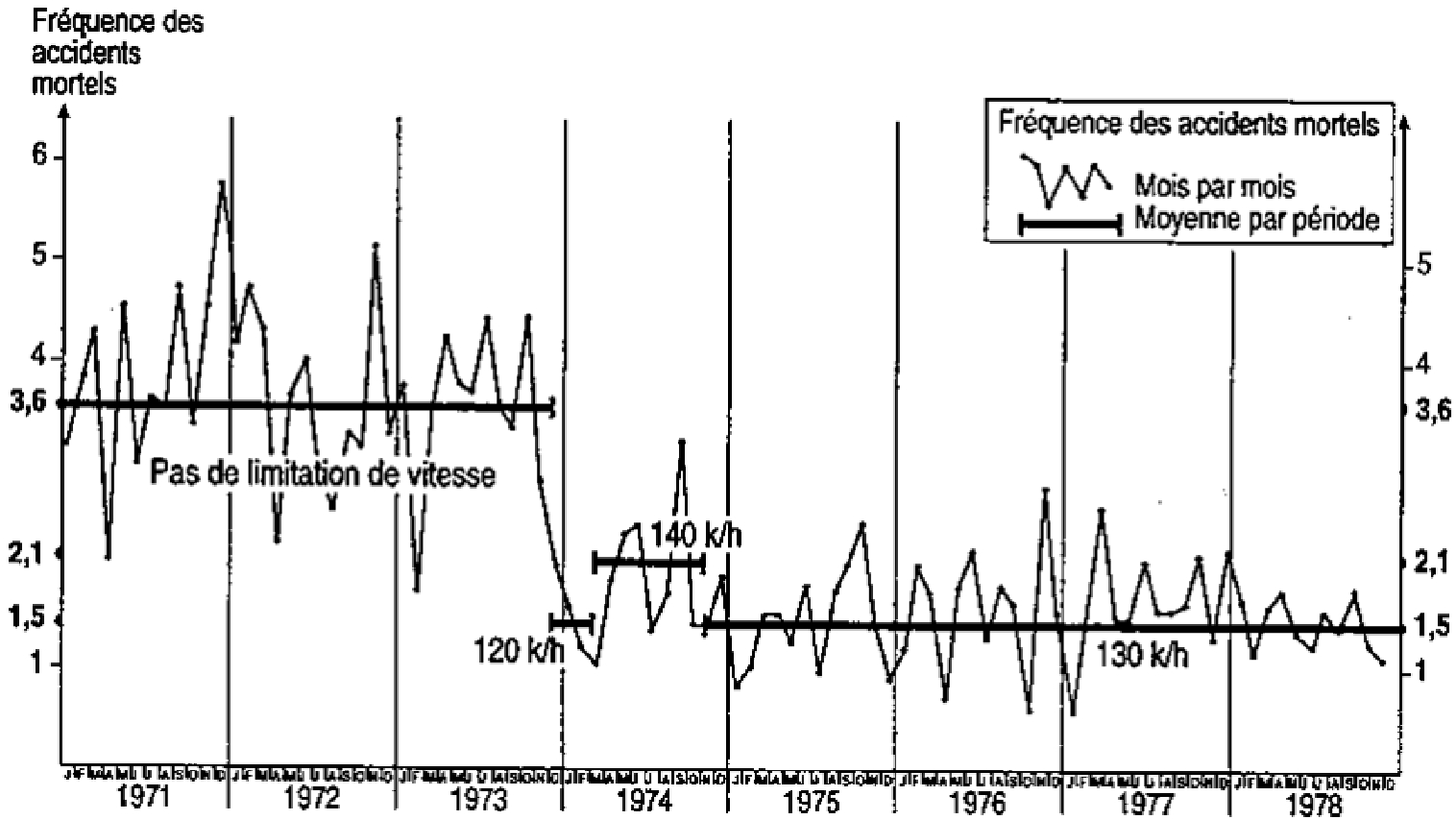
But why are many monthly model fits as published so good if they all include the year of the national or regional peak in fatalities? The (1956−1993) DRAG-2 model includes 1973 for Quebec; the (1968−1989) SNUS-2.5 model^[33,34] includes 1972 for West Germany; the (1957−1993) TAG-1 model^[35−37] includes 1972 for France, etc. Crucially, all such monthly DRAG-type family models include stationary multiple-order autoregressive schemes which explicitly bring in as regressors the order-lagged values of the dependent and explanatory variables, thereby implicitly transforming static models into dynamic ones^[38]. Careful analysis of their residuals reveals that, if and when they overshoot somewhat immediately after the occurrence of their global maximum, they recover rapidly afterwards. [This was also often confirmed at INRETS in Arcueil, France, during the summer periods of 2001 and 2002, by visual analyses of fits in Sylvain Lassare's ARIMA models of fatalities in France, using few or many dummy intervention variable shifts. Clearly, interventions modelled by such dummy variables never induce turning points (cf. Fig. 1)].

Figure 1. 

Effect of three speed limit changes on the frequency of fatal accidents on French highways^[39,54].

Fitting yearly models without the presence of intermediate economic output indicators

If monthly models of single regions containing intermediate and final output indicators (10 in DRAG-2, listed in Table 1; six in SNUS-2.5; 5 in TAG-1, etc.) easily 'miss' the presence of a global maximum by surfing gently over it, as it were, yearly models devoid of intermediate activities will notice the presence of a peak by failing to fit it both visually and parameter-wise. This occurs with Smeed's model, limited to the scale indicator Motor vehicle availability N, but also with models using N-km or real GDP instead.

In the beginning, there was no global yearly peak

Let us see how. In his first piece from 1949, Smeed^[13] (cf. Table 2) used Vehicles and Population to explain fatalities for a 1938 cross-section of countries by a simple logarithmic relationship amenable to slope estimation with a slide rule and graph paper. His famous equation S-1 was obtained by a log-linear adjustment (S-1 to S-4) between the yearly number of killed individuals per registered vehicle and the number of Vehicles per capita for 20 countries, a data set that included the 17 points shown in Fig. 2. He also declared himself satisfied with how the relationship fitted Britain for the 1909−1947 period^[40,41] and in tests with a sample of 68 countries for the period 1957−1966^[14,15]. [Discussing at Université de Montréal in 1973 or 1974, Smeed himself said he did not know why his relationship 'held']. Adams^[40,41] retested it for 62 countries in 1980 and was himself satisfied that the slope coefficients had barely changed from those of (S-1/S-4), but he provided no numerical estimates or t-tests, only graphs of fitted lines. He then claimed that, S-1 holding, safer driver-vehicle-way triplets clearly had no role in the explanation of the most recent road death numbers: drivers must just have re-established their risk at its previous level, chosen before triplets of new 'safety clothes' had been forced on them.

The breakdown of Smeed's relationship

We retested it with one of Smeed's data bases, S-5, and again with another, much more recent, pooled S-6 sample for which the estimated coefficient of the first variable changes sign (cf. Table 2), demonstrating clearly that the relationship breaks down. Detailed analysis by many^[42,43] indicates that failure happens in the mid-1970's as the model (S-1)−(S-4) starts to grossly over-predict fatalities in advanced countries. To see how this could occur, compare the data set for 1938 from S-5, found in Fig. 2, with that found in Fig. 3 that also includes pre-war values for 1931 from Smeed^[13] and from the S-6 sample.

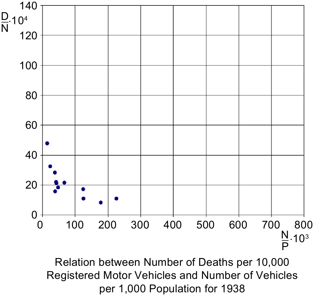
Figure 2. 

Fatalities per vehicle and vehicles per capita (Smeed's 1938 data in S-5 sample).

Figure 3 contains data for all 26 countries, for the years 1931 and 1938 together and for 1965, 1970, 1980, 1990 and 1998. Shown chronologically in Fig. 4, the film reveals clouds of points gradually moving down to the right and collapsing to a straight line approaching zero. Note also that all (red) points from S-5 (for 1931 and 1938) are to the left of 230 vehicles per 1,000 persons indicated on the x-axis but that (blue) points from S-6 (for 1965; 1970; 1980; 1990; 1998) are more evenly distributed.

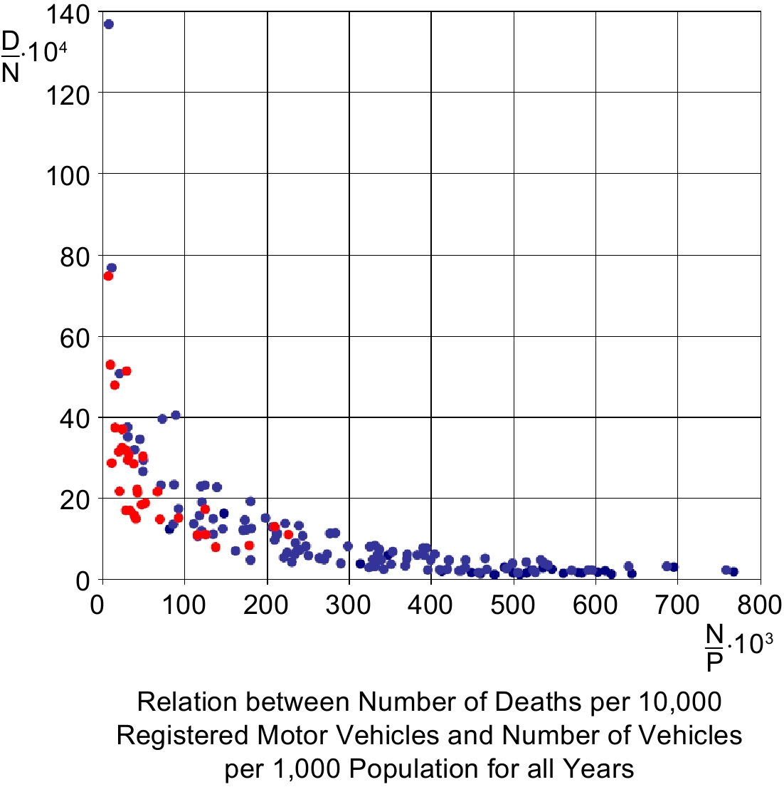
Figure 3. 

Fatalities per vehicle and vehicles per capita (Smeed‘s 1931; S-5 and S-6 samples).

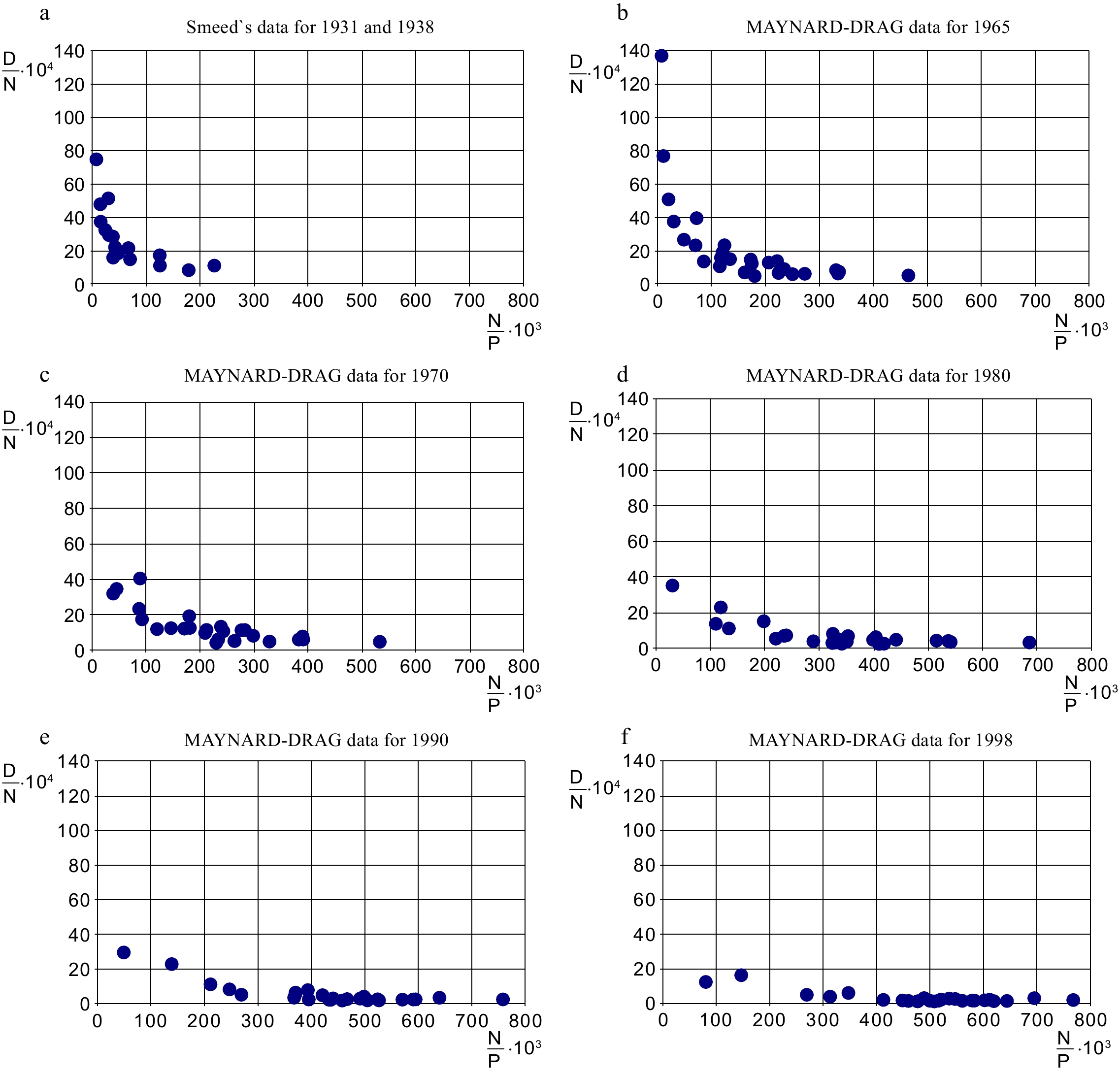
Figure 4. 

Fatalities per 10,000 vehicles and vehicles per 1,000 inhabitants over time in 26 countries.

Clearly, changes happen over time and it is strange to claim for the USA (cf. Fig. 5b also) that 'death rates due to motor vehicle traffic appear to be largely independent of the number of vehicles in circulation and stable [Marchetti's own data for the USA show variation from 16 to about 32 with sharply falling variance over time between 1920 and 1990 ─ hardly, as stated in his Fig. 15, 'a basic instinct in risk management' ─ to say nothing about accident rates in aviation where the view of any anthropological constancy across cultures or civilisations would be no less preposterous] around 22 per 100,000 inhabitants since Henry Ford's times'^[44].

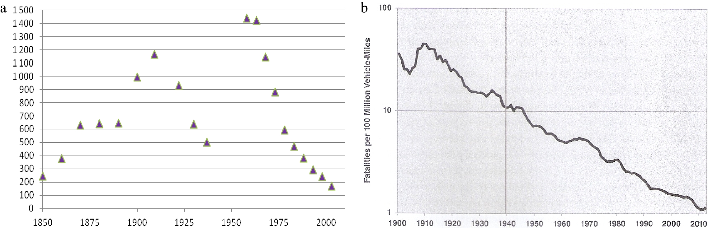
Figure 5. 

Secular fatality intensity of road traffic in France (1845−2005) and the USA (1900−2012). (a) Index of the fatality intensity of total road traffic. Deaths caused by horses, horse-drawn carriages and automobiles in France, 1845−2005 (mostly quintannual) (Source: ^[45], Figure 4.F, p. 14). (b) Logarithm of motor vehicle road deaths per 100 million vehicle-miles in the USA, 1900−2012 (yearly) (Source: ^[46], Figure 11-6, p. 386).

Bad dreams of imagined anthropological constants aside, the reason for the over-prediction in some 18 countries from about 1975 onwards is in fact that their fatalities stopped increasing and started falling, after having reached a global maximum between 1970 and 1974 (nine of which, listed in Table 4, are in 1972 alone) as indicated in Fig. 6. This clustering of maxima (the other maxima listed in Table 4 are less concentrated), at first diagnosed as 'The Mystery of 1972−1973'^[47,48], was later relabelled 'The Matterhorn' peak [Meadow (English) or Cervin (French)]^[13,49].

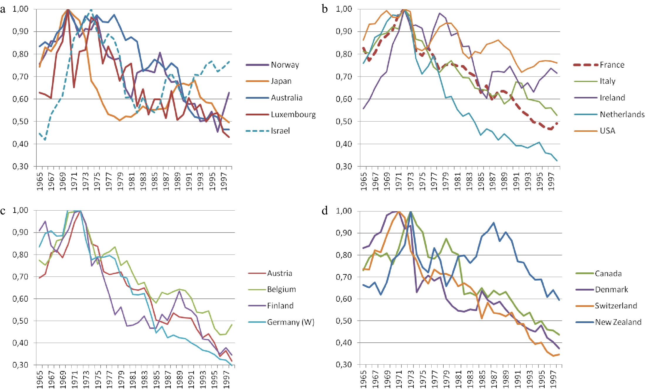
Figure 6. 

Meadow-shaped evolutions of yearly road fatalities in the 18 OCDE lustrum countries. (a) Fatality indices, 1965−1998: Norway, Japan, Australia, Luxemburg (1970 = 1.00), Israel (1974 = 1.00). (b) Fatality indices, 1965−1998: France, Italy, Ireland, Netherlands, USA (1972 = 1.00). (c) Fatality indices, 1965−1998: Austria, Belgium, Finland, West Germany (1972 = 1.00). (d) Fatality indices, 1965−1998: Denmark & Switzerland (1971 = 1.00), Canada & New Zealand (1973 = 1.00). Source: Gaudry^[51], except the series for Israel from www.cbs.gov.il/publications16/acci15_1643/pdf/gr01_e.pdf.

From 18 to 26 country maxima

If one extends this 1970−1974 lustrum time window in both directions, the number of fatality maxima increases to 26, as show in Table 5. Interestingly, analysis of monthly data shows that all 1972−1973 peaks occur well before the first oil crisis of October 1973, typically in late summer or early autumn. In fact, the global national maximum is reached by nine countries during the same quarter of 1972 and by two more about a year later, which raises the question: can these 11 peaks within 15 months be a random result?

In the above sections, we were on purpose slightly vague about injured road victims warranting medical care. To the extent that economic activities critically determine total traffic levels, they should be expected to peak at the same time as fatalities, but this expectation is muted by the possibility that they can also act as substitutes in a multi-commodity (deaths, injuries, material damages only) demand system of accident frequency or of their damage outcomes. Injuries might also increase their share when interventions aimed at extreme or risky behaviour, or when high congestion, exist, or when the final private (final) consumption share of traffic, as identified in Transport Satellite Accounts^[52], sharply increases after the peaking of Road traffic intensity of GDP.

But there is a greater difficulty still with injuries, linked to their general underestimation and to changes in police accident reporting procedures (always less thorough than coroner analyses of traffic deaths) calibrated without benchmarks and very differently across countries and motor vehicle insurance systems, as the analysis of Table 4 data demonstrates. [Quebec was considered by itself and added to the sample at the request of a principal funding agency in 1999−2002, Société de l'assurance automobile du Québec, then hoping an unambiguous road safety ranking indicator could be found].

International differences in the definition of road injuries

An examination of the per capita series of Appendix 2 confirms the well-known fact that the definition of a road fatality varies much less across countries than the definition of a road injury. Consider the values for the end of our series, 1998, reproduced in two columns of Table 4. Whereas the ratios of the maximum to the minimum for fatalities is 3.6 [= (Portugal = 2.1)/(Great Britain = 0.6)], it is 10.6 [= (USA = 118)/(Australia = 11.1)] for injuries. Although slight differences in the way fatalities are reported by the police (mainly due to the number of days of hospitalization considered to decide whether a road victim deceased, e.g. 1 d, 3 d, …7 d) may be consistent with a ratio of 3.6 that reflects real differences, there is no way that injury rates can vary by a factor of 10,6 across extremely similar countries (for instance the USA and Australia, that differ merely by a factor of 1.6 in fatality rates).

In addition to the levels of individual fatality and injury risk in 1998, it is interesting to note in Table 4 the evolution of these indicators since the dominant peak year (1972): the median and mean values of the fatality rate are 1.06 and 1.15 and those of the injury rates are 36.23 and 44.72, respectively. Since 1972, the percentage changes of both indicators exhibit variations that are in no way parallel, as the changing ranks of the 26 countries demonstrates: only Eastern Germany remains 25^th on both speed counts calculated over the 26 years 1972−1998.

Our position

Considering only the 18 countries with fatality peaks during the 1970−1974 lustrum, nine have their injury peak either simultaneously with their death peak (the five whose injury peaks are shown in Fig. 7a) or within 2 years before it (the four whose injury peaks are shown in Fig. 7b); the other half all have them after their death peaks, as can be verified in Appendix 1. Note already in Fig. 7, even before consulting Table 4, that the downside slopes of the injury indices of countries with injury peaks occurring earlier than their death peaks (in Fig. 7b) are on average lower (and more grouped) than those of countries with simultaneous death and injury peaks (in Fig. 7a), a difference that also requires explanation and suggests again the presence of a shared structural economic factor change.

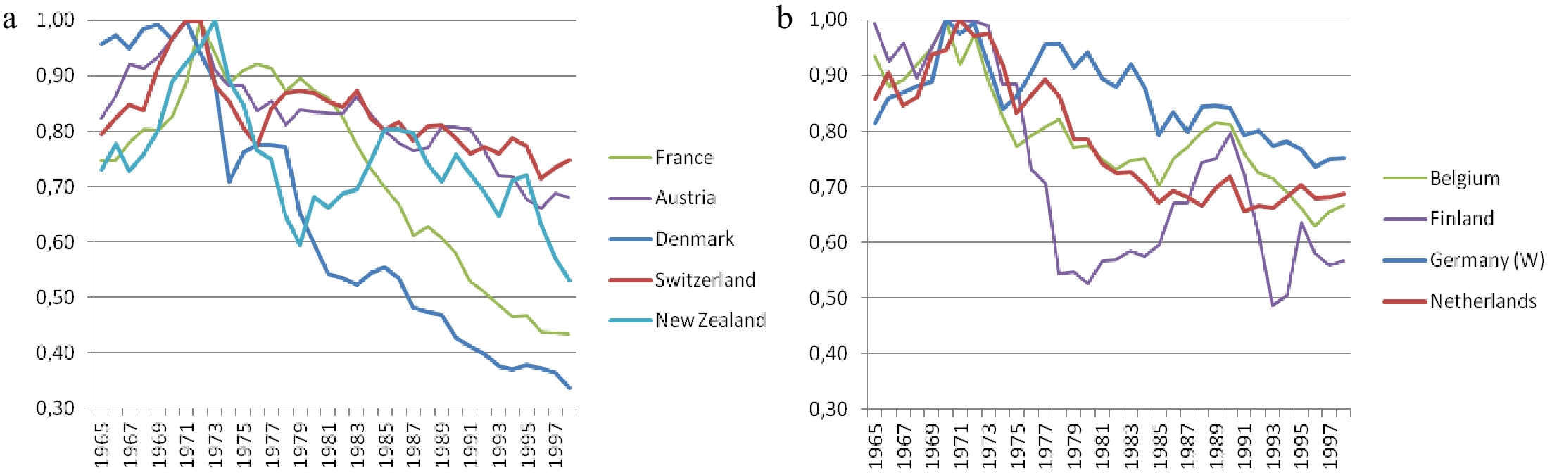
Figure 7. 

Lustrum country injury peaks simultaneous to, or preceding, their own fatality peaks. (a) Injury peaks synchronized with death peaks, 1965−1998: Denmark, Switzerland (1971 = 1.00); France, Austria (1972 = 1.00); New Zealand (1973 = 1.00). (b) Injury peaks occurring earlier than 1972 death peaks, 1965−1998: Belgium, Finland, West Germany (1970 = 1.00); Netherlands (1971 = 1.00). Source: all series are from the MAYNARD-DRAG database^[50].

Considering now only the 13 'regions' used in the regression models specified seven below (on 12 countries and Quebec), one notes that (i) seven of them will have synchronous fatality and injury peaks [Those of Fig. 7a except for New Zealand, plus Great Britain (in 1965−1966), Sweden (in 1969) and Spain (in 1989).]; (ii) three will have earlier ones [those of Fig. 7b, except for Finland.]; and (iii) three later ones [Norway (in 1977), Quebec (in 1979) and Canada (in 1989)]. We will not try to understand why some (a minority) of our model sample countries have injury peaks that are not synchronous with the fatality peaks: we just hope that the new I variable, Road traffic intensity of GDP, improves the fit for injuries as much as it does for fatalities ̶ slopes, leads and lags included. Concerning Denmark (in Fig. 7a), for instance, the downward trends of monthly accident aggregates of three categories (with killed, with seriously injured and with any injury victims) have been studied in depth by an author^[5] who concluded to the failure of all explanations based on recorded variables (exposure, GDP, etc.) over a long period (1978−2001). A better fitting model should mean gains in the quality of adjustment for all categories of safety performance measures and over their full sample ranges, and not just at Matterhorn period peaks.

Methods: on previous attempts to make sense of the 1970-1974 peaks, and intuition of the new variable I

Before we propose our own tests, it is useful to recall how people have tried to make sense of the 1970−1974 peaks, and even of their clustering, and to intuitively document the role of a new Road traffic intensity of GDP variable I for aggregate models where final activity GNP is already present.

On past attempts to conquer the Cervin/Matterhorn/Meadow

First, we survey in turn the main approaches used to explain the existence of Fatality peaks since the demise of Smeed's S-1 estimate:

i) Reductions in maximum legal speeds. It is tempting to impute a turning point to a reduction in maximum speeds (or to more belt use), but this linkage is dubious for reasons of both timing and experience with such interventions, which shift trends but do not cause them to turn.

Considering solely countries where fatalities peaked in 1972, Finland imposed reductions during that year but France only in March 1973 outside of built-up urban agglomerations (and in December for highways ̶ 'autoroutes') [In July 1973, the obligation to wear belts in front seats was combined with limitations to 110 km/h on high traffic roads and 100 km/h on the rest of the network] and the USA in March 1974. More significantly and decisively, such changes tend to induce shifts, not turning points, as in Fig. 1 where the legal maximum on the large French highway network changes thrice within 11 months [to 120 km/h on 3^rd December 1973; to 140 km/h on 13^th March 1974; to 130 km/h on 6^th November 1974].

If journalists all too easily make the linkage, for instance in France^[53], professionals may also succumb in light-hearted editorials void of due statistical tests^[39];

ii) Driver stock quality and congestion. Among structural variables other than speed limitations (combined with front seat belt use, or not), two candidates were examined and rejected^[55].

First, the 'youth bulge' theory^[56−58] whereby the wave of baby boomers would reduce the average quality of the stock of drivers, fails because its maximal impact on the average quality of the stock occurs only around 1980 in all countries concerned (Spain excepted), as young drivers of the baby boom obtain driver permits and progressively lower the average quality (based on relative risk by age) due to their exceptional cohort shares.

But the congestion theory, whereby OECD countries with fatality peaks in 1972−1973 often saw shares of public investment expenditure on highways fall after 1966, is a more credible prospect. It is noteworthy that a relative disinterest in roads occurs long before the strong increase in vehicle ownership that starts in 1970 (as baby boomers turn 22−23 or so), causing clear 10° to 15° kinks in national vehicle ownership trends and perhaps prompting OPEC to raise the price of oil in October 1973 on the background of a 4-year long bout of strong upward market pressure.

However, testing that congestion hypothesis is extremely difficult. Aggregate nation-wide congestion indices are extremely rare and consist mostly in single-year and single-country cross-sectional estimates^[59], not in long time series sufficient to suggest or back simultaneous turning points around 1970−1974. And, when series are available, they pertain to the higher network, as in France where average speed on it has tended to increase between 1967 and 1997^[36]. The only model containing a proper congestion index is TRULS-1^[60−62] estimated from a panel data set (of 5016 monthly observations on the 19 counties of Norway, 1973−1994), which contains the variable Vehicle-km per km of road per month per county but unfortunately does not start early enough to cover 1970, year of maximum Fatalities in that country;

iii) Victim mix and de-pedestrianization. Is it possible to explain maxima in road victims by a change in the mix of say pedestrians and others sharing the road? Some^[23] explain part of the decrease in numbers of persons killed since 1963 in 32 countries by the lower number of pedestrians killed; and similarly, with much hard work, an author^[20] extends the exercise to all combinations of road user interactions in The Netherlands. But these approaches fail to justify any turning point in aggregate Fatalities;

iv) Safer vehicles and ways. Safer vehicles and roads are often presumed to have favourable effects on safety and to yield a net gain despite some offsetting behavior to maintain a chosen risk level. The gain may be due to limits on risk taking: for instance, lighting is installed on highways but speed limits prevent users from maintaining their desired risk level. We know of no study of this undemonstrated presumption that could convincingly claim to account for even a single national maximum, to say nothing of the cluster of almost simultaneous turning points in 18 countries;

v) Imposed turning points. As the data obviously contain them, in many cases with different slope trends before and after the maximum^[63] [They examined Denmark, the United Kingdom, the Netherlands, Norway, Sweden and the USA], why not model turning points and preferably different before-and-after slopes? A first method consists in multiplying the growing indicator of interest by an exponential or logistic function of negatively weighted time, per force eventually yielding a maximum or a marginally decreasing value, depending only on the particular function and parameter of time. A second method, more amenable to yielding an asymmetric inverted U-shaped curve, fits a continuous non monotonic function, or fits splines, to a chosen structural variable, such as Vehicle occupancy or GDP per capita, as we presently see.

Concerning the first approach, for instance, some researchers^[22,64] notice the 1972 peaks in 4-5 countries (The Netherlands, the USA, West Germany, the UK and Japan) and fit the data by making the safety indicator follow a negative exponential function of time and traffic a sigmoid logistic one. The first author^[21] performs a similar exercise for road death peaks of 1972−1973 in the same five countries [For the UK, he neglected both the higher post-war value of 1966 (7,985) ― he uses 7,763 for 1972 ― and the true maximum in 1941. This sloppiness reduces his set from six to fove countries (keeping Israel that in fact peaked only in 1974)] plus Israel. But these exponential functions have zero asymptotes and are incompatible with current reported numbers of road casualties in developed countries^[65]; moreover, mere functions of time provide no structural explanation but just curve fitting.

With the second approach, one looks for a variable that could have non monotonic effects and one applies a procedure to estimate its shape as part of the regression model. A first procedure to test the ∩-shape uses two Box-Cox transformations (BCT) on the chosen variable W, usually within a regression model where BCT are used on the dependent and other variables, namely:

where the BCT is defined as:

and one of the explanatory variables, say W, is used twice as follows:

in which case the BCT are distinct [${\lambda _{Q1}} \ne {\lambda _{Q2}}$] and the model is identified in terms of transformed variables. In equation (3), the usual alternating signs conditions on ${\beta _{Q1}}$ and ${\beta _{Q2}}$, deciding if and whether a maximum or a minimum occurs with a quadratic specification, generalize to those listed in Table 6 where a given sequence of signs yields a maximum or a minimum depending on the sign of the difference [${\lambda _{Q1}} - {\lambda _{Q2}}$]. One might focus on the most general asymmetric turning case [$ {\lambda _{Q1}} \ne {\lambda _{Q2}} $], or on a particular one [${\lambda _{Q1}} = 1;{\lambda _{Q2}} \ne 2$], or even on the symmetric textbook quadratic [$ {\lambda _{Q1}} = 1;{\lambda _{Q2}} = 2 $], both nested in equation (3), to test existence and symmetry of the ∩-shape.

In monthly models, an asymmetric form [$ {\lambda _{Q1}} = 1;{\lambda _{Q2}} \ne 2 $] has been applied with some success to Vehicle-km in accident frequency and severity equations^[22,64]. However, in yearly models, it was applied^[19] without any success to the inverse of N/Pop, Vehicle occupancy (Population/Vehicles) within the authors' MnM-1 model, and they concluded that an adequate test with that variable would require country-specific forms, almost impossible to estimate in a pooled data set of 12+1 countries when a number of other variables are also subjected to BCT, as in the MnM-2 specification to be adopted below.

A second procedure to obtain ∩-shapes uses splines^[67] on the Income variable (defined as GDP per capita) with a 1963−1999 panel data set for 88 countries. The authors' piecemeal linear approach to explain fatality rates (with 10 income groups, each having the same number of observations) was used on logs of Income, which allows the monotonic logarithmic function pieces to turn. This involved 10 different spline coefficients whereas using two BCT as in the first procedure would have involved only four parameters (two coefficients and two BCT powers). The rest of their otherwise sparse model consisted in eight (linear or logarithmic) regional time trend variables (for seven geographic and one high-income country groupings).

Their estimated turning point Income per capita is $8,600 (in 1985 international dollars), 'after which the fatality risk begins to decline'. This is a very low number if one looks at the per capita income of the countries listed in Table 4 during the year of their turning point, as documented in Table 7. Only the UK turns at that income level and countries can turn at much higher values or at much lower ones (note Portugal and Switzerland, the lowest and highest). Indeed, the standard error of actual turning point values is greater than the per capita GDP of many countries!

Clearly, a dollar of income does not have the same rough transport safety implications in the different countries and something is obviously missing from the Income-only explanation of the turning point: Greece, Luxemburg and Iceland, to say nothing of the others (the relative standard error of income for the year of the maximum is 0.4), turn at too different income levels. One suspects that something physical should complement the GDP dimension of final output in value, even if one has used splines which are more flexible than a straight quadratic [A quadratic specification of per capita GDP, imposed to explain Algerian fatalities (which have yet to exhibit a visible global maximum) is too violent^[68] and would no doubt have been rejected in a test with equation (3)]. A presumed advantage of the intended addition of the Road traffic intensity measure I is the introduction of a physical dimension to characterize economic development, because a given GDP per capita money value may correspond to quite different (intermediate and even) final output basket mixes.

The idea of Road traffic intensity of GDP

The idea that I, Road traffic intensity of GDP, with a numerator reflecting flows derived from all activities, complements GDP already included as determinant of death levels and rates in yearly models was prompted by graphs of I for the USA^[69] (where fatalities peak in 1972) and comforted by graphs for Norway (where fatalities peak in 1970). Both sets of graphs, reproduced in Fig. 8, point to a role of I in explaining the Fatality peaks.

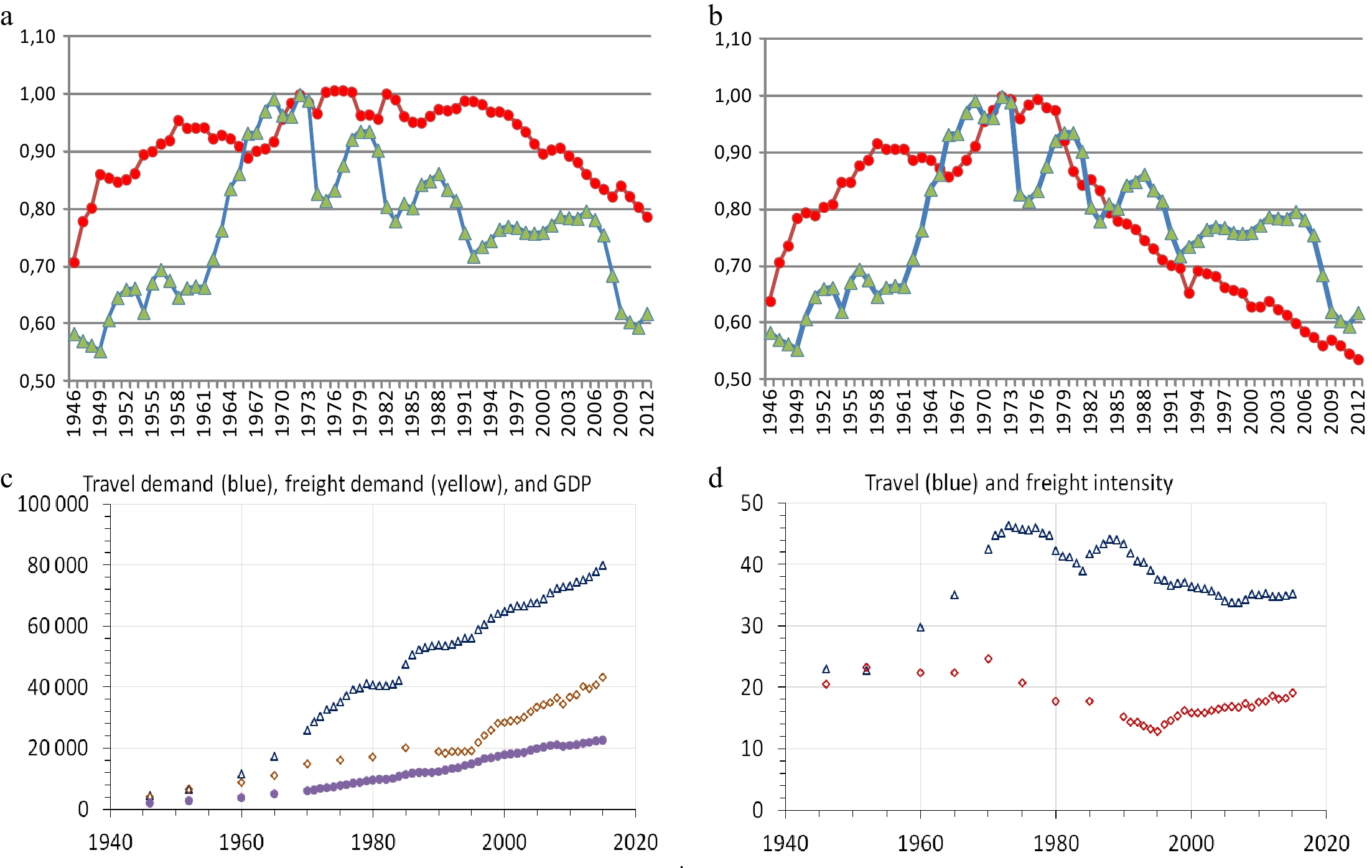
Figure 8. 

Measures of national transport intensity of GDP (in constant national currencies). Upper pannel, Fatality (1972 = 1) and Road traffic intensity of GDP indices (1972 = 1) for the USA, 1946−2012. (a) [Fatalities () and] Mile intensity of GDP (). (b) [Fatalities () and] Gallon intensity of GDP (). Lower pannel, Norwegian GDP and all-mode transport intensities, 1946, 1952, 1960, 1965 and 1970−2015. (c) Domestic travel-km & freight-km and GDP in Norway. (d) Travel & freight transport intensities of GDP in Norway. Sources: ^[69] for the Mile and Gallon intensities of GDP (); NHTSA Safety Facts (Various years) for Fatalities (). Lower pannel source: Lasse Fridstrøm. Produced on 22^nd October, 2017.

The link between I, the Road traffic intensity of GDP, and the profile of peaking Fatalities is in fact obvious for the USA for which the author^[69] defines two 'measures of the relationship between road transportation and economic activity', both presented in index form in upper pannel of Fig. 8, but fails to link them to the 1972 peak in American road fatalities (plotted here with each measure). Although he does not use the expression 'traffic intensity of GDP', he effectively calculates it with Vehicle-mileage (T1, which peaks in 1977) and with Gallons of fuel consumed (T1*, which peaks in 1972). Interestingly T1, which is actually more correlated (0.62) with fatalities than T1*, is logically and statistically the best candidate for a traffic intensity of GDP linkage to fatalities. But what of Norway?

Although lower pannel of the graphs in Fig. 8 pertain to all modes [The data pertain to domestic transport only and exclude the non-motorized travel modes (cycling and walking) and use of international travel and freight. Globalization has probably moved abroad a growing share of transport in recent decades], the overwhelming road share in these series suggests a peak in road transport intensity around 1970, year of maximum road fatalities. The changing composition of the economy is hard to detect with absolute levels of traffic and GDP in the left-hand side Graph A but comes out clearly in the right-hand side Graph B. And the distinction between freight and passengers enriches the link between economic development and the transport intensity of GDP (if not directly its specific road transport intensity) but should still allow changes in their sum, peaking with fatalities in 1970, to mimic changes in the ratio of intermediate to total output.

In short, in the absence of yearly aggregate data series on intermediate output, the new variable seems to be the simplest way to introduce that sort of economic structural change into yearly models, even if more sophisticated ones could be imagined if appropriate yearly data were available by country. The new variable I (to be defined more precisely) resembles the Transport intensity of GDP notion^[70] but has different units from it because we are interested in the road mode and not in the sum of all modes.

Putting flesh on I, the yearly indicator of road transport intensity of GDP

But how should I be measured? Figure 9 presents an apparent dilemma because the fuel consumed measure matches peaking fatalities in Norway, as in the USA [In Belgium, Denmark and the USA, the fuel consumed-based indicator profile is somewhat closer to the Meadow-shaped profile of road fatalities than the distance-based measure], but it is the distance-derived measures that provides the same match in France. We shall use the latter measure of I, the correct one, which has a correlation of only 0.60 with the fuel measure over our sample period 1965−1998 of vehicle fuel efficiency gains [In upper pannel of Fig. 8, the correlation between the two indices for the USA is only 0.16. Vehicle fuel efficiency gains become a concern only after the first OPEC shock of October 1973].

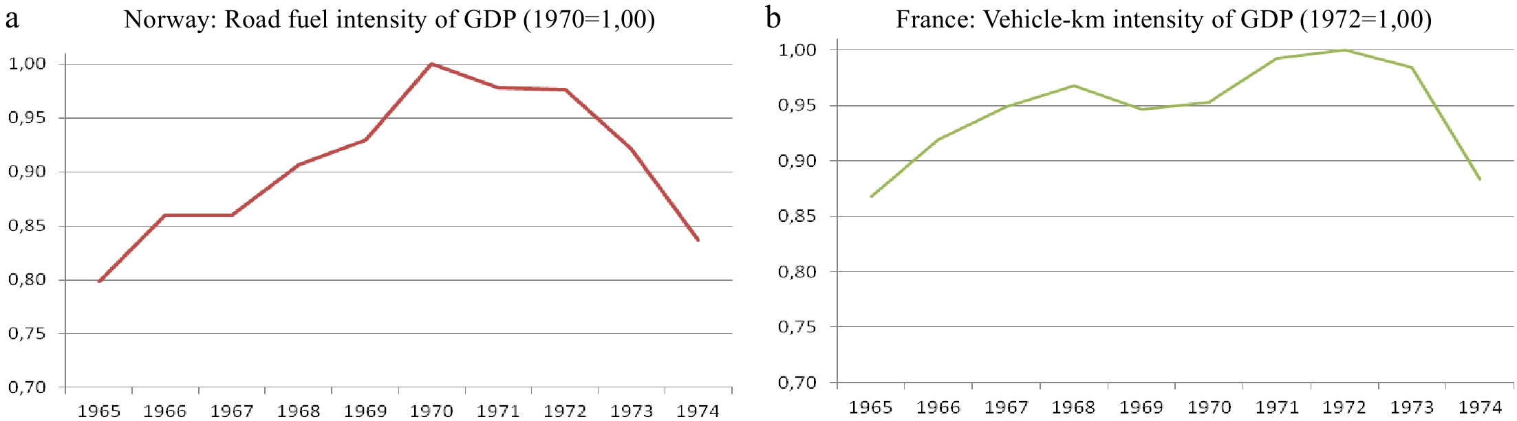
Figure 9. 

Road fuel and Vehicle-km indices of road use intensity of GDP (defined over 1965−1998). Source: all series are extracted or derived from the MAYNARD-DRAG database^[41] except for the GDP series for France, which is from INSEE. The traffic intensity indices are defined over the period 1965−1998.

On the evolution of I 1965−1998

To introduce the notion of Road traffic intensity of GDP above, we have calculated our indices over the period 1965−1998 and shown, in T1 of Fig. 8 and in Fig. 9, portions of those indices that happen to reach their global maximum of 1.00 synchronously with fatality indices. But this conjunction is secondary: a valid enrichment of the initial model by the addition of I does not require that this measure reach its maximum at the same times as fatalities. In fact, measures of I often exhibit only a weak local maximum (and not a global one, as they increase further) at the same time as fatalities, as is the case in Fig. 10 for Denmark and The Netherlands, included in our estimation sample of 12+1 countries, as well as for Finland and Italy, which are not.

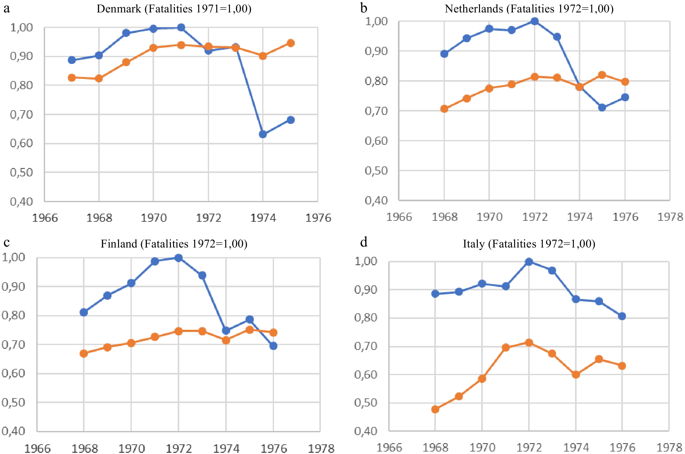
Figure 10. 

Global maxima of fatalities (at 1.00) and local maxima of road traffic intensities of GDP.

I as having induced regional convergence in regional per capita incomes?

A significant maximum in the transport or traffic intensity of GDP is a profound economic change. Note that GDP growth rates by region seem to diverge in the USA since about 1972 and GDP growth rates by worker since about 1980 when rates in coastal states take off relatively to rates for non-coastal regions^[71], ending the great post World War II convergence in regional per capita incomes.

These new divergences among American regional growth rates could reflect the evolution of the national ratio of intermediate (or total) to final output that accompanies the start of the decreasing Road traffic intensity of GDP in the USA in 1972.

On I as an economic spine for natural hill-climbing without splines

Our equation specifications below purport: (i) to enrich the description of economic development activity variables by adding Road traffic intensity of GDP to GDP per capita; (ii) to make no changes in the other variables, be they socio-economic (age and vehicle shares, urbanization, etc.), or climatic (average temperature and total precipitation) and perhaps subsumed in constants or in trends, dominant in some authors^[17,67], especially when, like the latter authors, one resorts to intuitive country groupings manually defined a priori (i.e. not endogenously within the model). Trends, linear or turning, are not proper behavioural variables but signs of desperate model specification poverty, of modeller ignorance, or of both.

Is the Matterhorn sub-period of I atypical?

After specifying our equations and reporting our results, we will probe the background of The Matterhorn 1970−1974 period of interest. We will see that it is an exceptional period of worsening fatalities and fatality rates per kilometer driven that requires some reconciliation with a secular background of apparently decreasing Fatalities and Fatality intensity of traffic. It may then be that Road traffic intensity of GDP can help to understand not only the exceptional contrary periods of peaks (including that of the post-Great Depression in the USA) but also the downward evolution of the Fatality intensity of traffic itself over the 20^th Century in both France and the USA. We will propose a tentative interpretative framework for this reconciliation, based on what is known of the secular behavior of the Fatality intensity of traffic in those two countries.

Selected model specification MnM-2: the frequency of bodily injury accidents, their severity rates and victims (1965−1999)

A context of fixed and flexible form modeling

Page^[72] takes after both Smeed's 1949 model of road deaths and Peltzman's 1975 model of road deaths and injuries in that, studying yearly fatalities with an international data set, he likewise uses the Log-Log regression form while increasing the number of explanatory variables from Smeed's 2 to 7 (Peltzman had 5 plus a trend). He also claims^[73] that the next decisive step in modeling after Peltzman occurred with the monthly DRAG-1 model of 1984, which included both multiple-outcome specifications (e.g. deaths; injuries by category; no injury), with those outcomes decomposed (e.g. between road use in vehicle-km, accident frequency per vehicle-km and severity per accident), and all equations estimated with Box-Cox transformations. But, despite his knowledge of the tradition of multinational specifications and of regression forms, Page did not try to model any maxima over the period 1980−1994 or to use flexible Box-Cox forms, which can also dominate fixed Linear and Logarithmic forms in yearly models (e.g. for the USA^[18,74,75]). On this point, there might be an unexplained difference between monthly models, where optimal forms are never logarithmic and yearly models, where they often are (like here).

Our problem statement

With that background and context, our problem is simply stated: if Vehicle-km kept increasing after the 1970−1974 peak of Fatalities (and of Injuries, most of the time) in 18 industrialized countries and if road use was barely affected by the oil crises of October 1973 and 1979−1981, why did Fatalities (and often Injuries) start falling, as in Fig. 11 showing sums for the 12 countries [Despite efforts, some variables found in the database are unavailable for some countries, thereby limiting the sample] retained for our tests? In it, note growth rates of the indicators over the period decreasing successively with Vehicle-km, GDP per capita, Injured victims and Killed victims. [This is of course in part due to the fact that 9 of the 12 retained countries, Canada included, have their maxima of fatalities during the lustrum years 1970−1974, the exceptions being the UK (1965), Sweden (1966) and Spain (1989). All countries that have a maximum of fatalities during lustrum years have simultaneous injury maxima, except Canada], in that order. Our regression sample period is always 1965−1999 and its content is always that of the 12 countries plus the Province of Quebec, all 13 of which are greyed in the first column of Table 4.

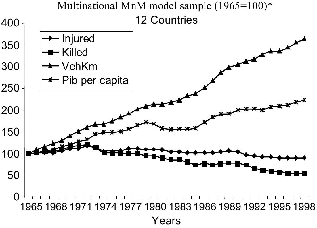
Figure 11. 

Indices of road use, GDP per capita, and killed or injured victims in our sample. * The 12 OECD countries selected in Table 4 (1965−1998 data).

A multinational model

To test the new hypothesis and obtain a natural, non-imposed, maximum from a naturally turning (non-monotonically increasing or decreasing) variable, we suitably modify the (multinational) MnM-1 model specification^[19] that previously failed to correctly account for fatality and injury peaks by inclusion of a turning form of type (3) on the Vehicle occupancy ratio (Population/Vehicle) explanatory variable.

Although Table 5 proposes much more than a dozen candidate countries for the estimation sample, and the documented MAYNARD-DRAG database is relatively complete for many countries, the latter does not cover all of the countries listed in the table (Israel, for instance) and may be incomplete for some countries covered. The size of the estimation sample will then depend on two model specification dimensions: the number of retained explanatory variables and the number of explained variables. Concerning the first, there exist for instance no Vehicle-km data for Luxembourg, Hungary or Greece; concerning the second, our desire to explain Morbidity and Injured victims rules out countries where the definition of injuries has notoriously changed (cf. Appendix 1), such as Australia (in 1979−1980) and the United States of America (in 1971−1972). One ends up with 12 countries (and Quebec).

Our MnM-2 specification, borrowed from that of MnM-1 to which the new I variable will be added, and estimated with the L-1.4 algorithm^[76] implemented in Version 2.0 of TRIO^[77], is consequently as follows:

i) The retained DRAG-type decomposition is: (Frequency) × (Severity) = (Victims). One then obtains five distinct equations: one for Accident frequency (the sum of fatal and non-fatal bodily injury accidents), two for Morbidity (Injured victims per bodily injury accident) and Mortality (Killed victims per bodily injury accident) rates and two more for the products of the frequency and severity terms, Injured and Killed victims. The application of Box-Cox transformations, in accordance with (1), to the dependent and up to five groupings of explanatory variables never led to really clear and significant gains over the logarithmic form, which was then retained for all equations, except for the significant heteroskedasticity correction (4) in some of the equations;

ii) The retained explanatory variables common to all five equations, listed in Table 3, belong to familiar categories in road safety models. We have added to category A our new Road traffic intensity of GDP variable I. Here GDP per capita is the key determinant of the demand level, in contrast with monthly DRAG-type models which use Vehicle-km (which here is uncorrelated (+0.01) with GDP per capita but is correlated (+0.90) with Road traffic intensity of GDP). When the inverse of Smeed's N/Population was added, it was never statistically significant and was not retained. An intercept guarantees invariance of BCT estimates to units of measurement of the X_k and Z_m^[78];

iii) Tests of heteroskedasticity were performed with^[79]:

and the Z_m variable Vehicle-km found to make a significant contribution in three of the five equations;

iv) For each equation, we have performed Box-Jenkins analyses. At first, of the existence and stationarity of the constant variance residuals v_t assumed to follow a multiple-order process

and, after correction, of the final residual w_t to guarantee that a white noise had been obtained.

Autocorrelation and heteroskedasticity have not been dealt with previously in multinational yearly models, although Page^[72,73] reported that he tended to obtain first differences (ρ₁ = 1 in (5)) in his exploratory trials and consequently assumed ρ₁ = 0 to avoid this predicament. We found some significant 1^st order estimates in three of the five equations, but no 2^nd order ones. Contrary to Page's result, all three of these 1^st order processes are stationary, but barely so with values of ρ₁ between 0.95 and 0.97;

v) The t-statistics of all β_k and δ_m were computed conditionally upon the optimal values^[80] of the BCT by a method of first derivatives^[81] that avoids unit of measurement and other rescaling pitfalls^[82];

vi) The tested specification for the five equations, for any given country $i = 1,...,13$ and period $t = 3,...,35$, was then:

where ${\beta _r}$ is the coefficient of the country-specific dummy variable of arbitrary reference region r;

vii) The optimal forms of ${\lambda _y}$ and of the ${\lambda _X}$, but not of the ${\lambda _Z}$, of the initial model of Table 8 were deemed approximately logarithmic after making sure that global maxima of the Log-Likelihood had been found^[83]. Second order autocorrelation was never significantly different from 0, and ρ₂ was finally set at 0. Page's first differences (ρ₁ = 1) in logarithms were rejected in most cases only by weak numerical margins but the estimated partial differences were retained as still the most likely values, sometimes even statistically different from 1;

viii) All results were carefully checked for robustness with respect to multicollinearity using Belsley-Kuh-Welsh^[84] indices as duly reinterpreted^[85];

ix) Neglecting region subscripts, the Rosett-Nelson^[86] model with Gauss-distributed $N \sim (\sigma _w^2,I)$ errors ${w_t}$ collapsing to the Box-Cox likelihood in the absence of limit observations on y is:

where $\left| {\partial {u_t}/\partial {y_t}} \right| = y_t^{_{{\lambda _y} - 1}}$ denotes the Jacobian of the transformation from the w_t to the observed y_t. We verify ex post the reasonableness of the assumption of normality with graphs and of the absence of limit observations by calculating an index of the probability of each fitted value to be at the limits (defined by the user). We report on this statistic in Part III of Tables 8 & 9.

The initial specification and its results listed in Table 8 are representative of yearly models principally because the variable GDP per capita is included as implicit generator of road demand, and therefore of accidents and victims. In Table 9, the newcomer I variable, Road traffic intensity of GDP, is simply added without any other change to the specifications. Results are in 3 parts:

i) Part I. presents elasticities of y and t-statistics of the regression coefficients. When the code name of the variable is underlined twice (for instance SeatBelt in Tables 8 & 9 or Country-specific Dummies in Appendices 4 and 5), the elasticity measure approximates, for a variable containing some null observations, the discrete percentage impact on y of the presence of the variable. The expressions used to estimate these discrete 'elasticities' are from a paper^[87] where a thorough 10-page summary of elasticity notions for all types of explanatory variables is found.

Note that all signs are reasonable, at least for the equations for Accident frequency, Injured and Killed victims for which we have anticipations, and no doubt correct for the two Severity equations for which sign anticipations are unclear: indeed, our sign intuition is typically more about accident frequency and victims than about severity rates. It is then very interesting to see how some variables, like the pair of population age share variables, can have their most important impacts on the severity of accidents and not on their frequency or victims.

In Appendices 4 and 5, the Average yearly temperature is a very significant factor in the explanation of the frequency of accidents and of the number of victims, a result which is consistent with results of monthly national time series models where temperature variations across months of the year are significant generators of similar outcomes.

As the number of victims by category is the product of the accident frequency by particular severity rates by category, the sum of their elasticities theoretically would equal the elasticity of the number of victims of that category if it were not estimated within its own equation. We therefore provide here two ways of making sense of the elasticities of variables on victims: directly estimated or resulting from the sum of frequency and severity elasticity estimates.

ii) Part II contains parameters estimated to compensate for heteroskedasticity and autocorrelation. Note that two t-statistics are supplied for the λ_z from (4): with respect to 0 and to 1.

iii) Part III lists general statistics, including maximized Log-Likelihood (LL) values and the selected estimation sample size [The sample for estimation starts at observation 27 because, with 13 regions and the 455 observations stacked by year and region (year 1, region 1,…, region 13 ; … ; year 35, region 1,…, region 13), estimation of second order autocorrelation in (6) requires use of the first 26 observations. Starting the estimation at observation 14, in view of the absence of second order autocorrelation, and thereby increasing the estimation sample by 3%, made little difference. Each year, the 13 region values appear in the same order (indicated in Table 4 and in Appendices 4 and 5)].

Summary of key results

Note in summary Table 10 that adding the variable Road traffic intensity of GDP increases the LL considerably (except in the Morbidity equation, a result neither expected nor surprising) and also clarifies the role of the GDP per capita variable, i.e. its elasticity and t-statistic.

The contribution of Road traffic intensity of GDP

The results gathered in Table 10 demonstrate that it is bad economics to neglect the role of intermediate output indicators, and to limit oneself to final output ones, in explaining national road safety performance for the 35 years of economic growth from 1965 to 1999. Although we cannot here expect the single yearly indicator I of Total to Final output activities to yield as refined a contribution as that of 5−10 distinct intermediate and final monthly factors used in monthly models, results obtained are still completely convincing. Indeed, the addition of I dramatically boosts LL estimates in all equations except that of Mortality (Column 3). It is noteworthy that the fit of Morbidity (Column 2) is so much improved, but we limit our supplementary comments on residuals to the more intuitive Accident (Column 1), Injured (Column 4) and Killed (Column 5) equation dimensions. For this, we look at ratios of residuals w_t before and after adding I.

Although residuals of any equation always have a mean of 0, by construction, the ratios of their initial to enriched values shown in Fig. 12 can tell us much about the source of LL gains imputable to the added I variable. LL fit notably improves by reducing some relatively high error values of the lustrum period: (i) in the equation for Accidents (Part A), the addition of I corrects mostly one-sided outliers, one of which, in 1971 (for Quebec), is 16 times higher before than after correction; (ii) in the equation for Injured victims (Part B), the addition of I corrects an error of 1972 that is 46 times higher than before the correction and another one of 1970 that is 30 times smaller (both of which pertain to The Netherlands); (iii) in the equation for Killed victims (Part C), the addition of I corrects residuals in both directions, one of which (for Norway) in 1974 is 37 times higher before correction.

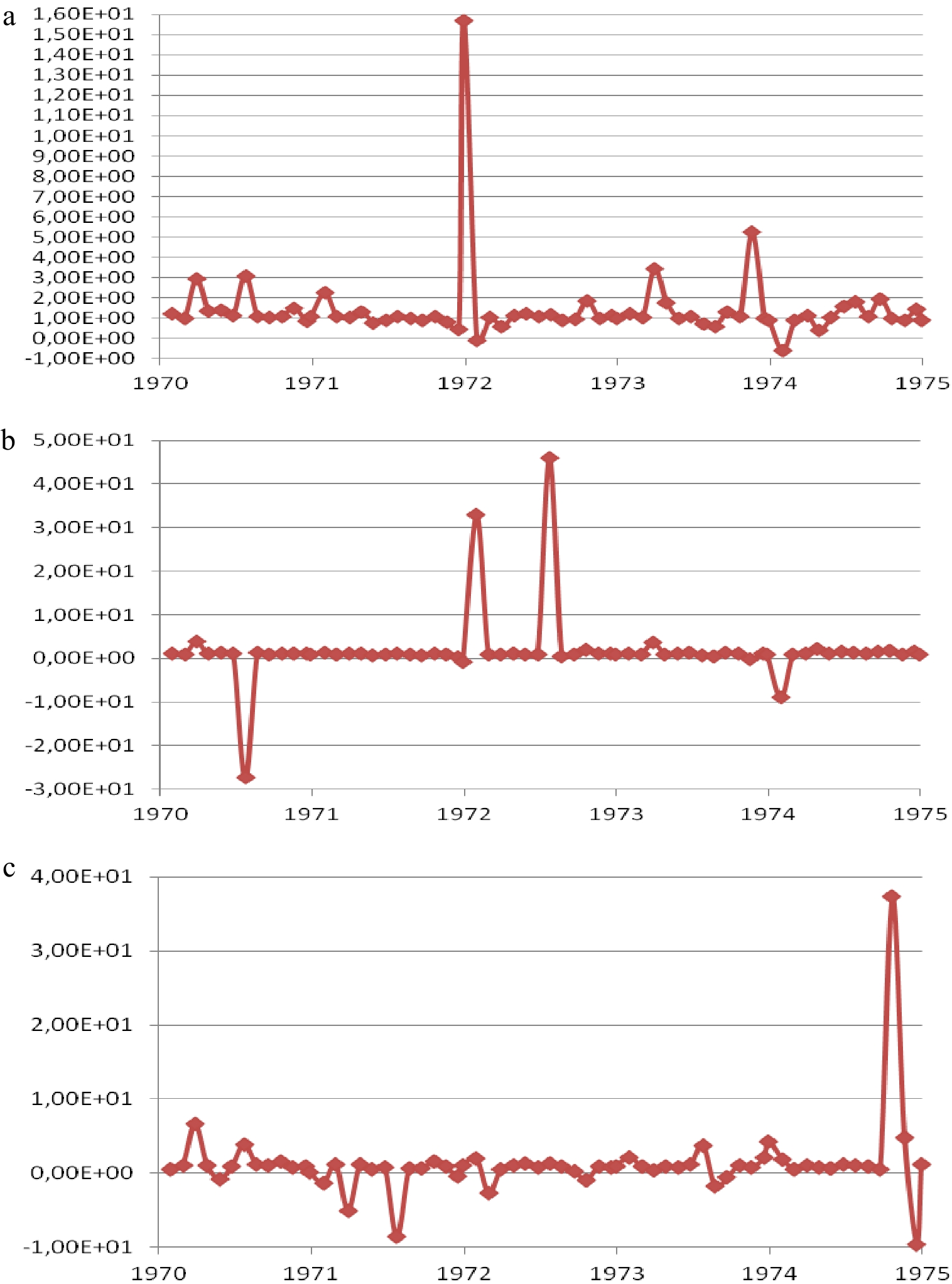
Figure 12. 

Ratio of initial to enriched residuals wt during the five lustrum Matterhorn years 1970−1974. (a) Accident equation, 65 observations for the Matterhorn period, 13 regions per year for 5 years (1970−1974)*. (b) Injured equation, 65 observations for the Matterhorn period, 13 regions per year for 5 years (1970−1974)**. (c) Killed equation, 65 observations for the Matterhorn period, 13 regions per year for 5 years (1970−1974)***. [* The average ratio of initial to enriched Accident errors values for the full estimation sample period (1967−1999) is 0.96. ** The average ratio of initial to enriched Injured errors values for the full estimation sample period (1967−1999) is 1.14. *** The average ratio of initial to enriched Killed errors values for the full estimation sample period (1967−1999) is 0.32.]

Discussion: lustrum period spurts in Fatalities and in the Fatality intensity of traffic

It is one thing to claim that, in the absence of the proper macroeconomic indicators of intermediate output activities constructed in monthly models to accompany final activity generators (cf. Table 1), yearly models have to do just with I, Road traffic intensity of GDP, at least during the post WW II years that include the clustered peaks in road fatalities, but it is another to claim that this proxy could be readily used on a secular basis in just the same simple way. On this, our lustrum period of interest, seen until now as a time of global national maxima of road fatalities, also needs to be positioned as a special sub-period bout with respect to some known evolutions of the Fatality intensity of traffic.

This statistic is available since 1845 for France and since 1900 for the USA, as shown in Fig. 5, where both indicators measure the Fatality intensity of road traffic, but for France the mostly quintannual data cover all road deaths (by horse or hippo-mobile included), in contrast with the yearly motor vehicle USA series (which excludes horse crash data). The share of horse-linked deaths (not shown in this figure) fell steadily from almost 100% in 1910 in the USA and in France, for which the source of Fig. 5a notes that it was still 14,85% in 1937, the average year for 1935−1940.

Neglecting road injuries warranting medical attention and remaining focused for simplicity only on road deaths, it is important to note first that the national peaks in Fatalities of Fig. 6, objects of our specific inquiry, also imply peaks in the Fatality intensity of traffic (in deaths per vehicle-km) during the same 1970−1974 period: they are clearly visible for both countries in Fig. 5.

Seeking an interpretative framework to distinguish between special periods and the long term

To discuss the positioning of our 1970−1974 spurt in both Fatalities and Fatality intensity of traffic, we distinguish two long periods, namely 1910−2010 and 1845−1910. Our problem is to set our sub-period of interest within its very long background and, in view of the lack of explanations for the trending evolutions over those long periods, to propose an interpretative framework whereby Road traffic intensity of GDP has more than a palliative role in explanations of secular fatality intensity indices.

Essentially, using I per force as proxy for the ratio of Total (intermediate and final) to Final output makes sense for the period of the post WW II peak in road fatalities of interest here [Although some authors^[88] included Miles as explanatory variable, yearly models, constrained by the absence of intermediate output measures, never conceived of, or estimated, distinct GDP and I effects proper. These could have been derived from log forms of GDP, Miles and the ratio of Miles to GDP in order to bring out, like us, the role of non final economic activities. All such models therefore implicitly assumed that intermediate output is proportional to final output.], as it would to explain the USA post-Great Depression surge, but the matter would be more complicated over long periods. To see this, assume that the information on intermediate output becomes available and that one can suddenly construct yearly ratios of Intermediate to Final, or of Total to Final, economic output.

Clearly, periods of fast industrialization may imply that both of these ratios of intermediate to final or of total to final economic output increase without much effect on I if mode choice and vehicle carriage capacity dampen, or go in the opposite direction of, impacts of macroeconomic structural change. Furthermore, the link between I and the Fatality intensity of traffic will depend crucially on vehicle density (congestion) on the road network. Consider the most recent long period of 1910−2010 first, for which there are reasons to think that congestion has increased progressively in France and in the USA, and contrast it to the previous 1845−1900 period for France for which there are grounds to think that congestion decreased in spite of strongly increasing intermediate to final economic output changes.

Bumpy 1910−2010 Fatality intensity of traffic trends

It is difficult to explain these two national declines in rates of more than an order of magnitude from 1910 to 2010 and there exists no real body of commentary on them, and naturally no consensus on how the diffusion of the automobile caused them.

To understand the difficulty, consider the USA where the death rate per mile of motor vehicles shown in Fig. 5b falls yearly by 3.6% on average between 1909 and 2012 but exhibits sub-periods of contrary upswings, such as the 1932−1935 post-Great Depression spurt and the big bulge of the 1960s. The author gratuitously imputes the fall of the index by a factor of 3 over the early period 1909−1926 to 'improvements in automobile quality and the first round of improved highways' (p. 386). This is unconvincing because the USA had a large high-quality network of paved roads before cars even appeared. In 1904, there were 154,000 miles of paved roads for 55,000 cars^[89,90], which amounts to about 100 times the amount per car to-day, because 'road infrastructure development preceded the diffusion of the automobile'^[70] (p. 127). Strangely, he is also silent on any changes in the structure of Total to Final economic activity associated with the visible post-Great Depression spurt and with the long 1960−1970 bulge, ignoring obvious trend reversals.

By his stated logic for the 1909−1926 drop, that last 1965−1972 surge should presumably be partly imputed to worsening automobile quality and worsened highways ̶ during the very decade of innovative safety regulation and diffusion for new vehicles (lap and shoulder belts; energy-absorbing steering columns, high penetration resistance (HPR) laminated windshields, padded instrument panels, dual braking systems) and of the deployment of the interstate highway system (1962−1969)!

And the argument that a large network of paved roads preceded the diffusion of the automobile can also be made for France, where the indicator in Fig. 5a also falls strongly after a rise from 1900 to 1910 resembling the American one during the earliest diffusion [Sales of Ford's Model T started only in 1908, with 5,986 units, and reached 260,720 units by 1913^[91]] of the automobile in both countries.

Basing the 1910−2010 trend on factors other than better driver-vehicle-way interactions

What is amiss if better vehicle-and-way incantations obviously fail to explain the trends since 1910? Could it rather be that, in both countries since 1910, progressively higher automobile traffic densities (congestion, reducing feasible speeds) [This role of congestion, understood as higher traffic density, is modelled in TRULS-1^[60−62] estimated from a panel data set (of 5016 monthly observations on the 19 counties of Norway, 1973−1994), by use of the variable Vehicle-km per km of road per month per county] on pre-existing relatively good paved roads and the substitution of automobiles for horses and their carriages (reducing vehicle heterogeneity and the much higher hippo-mobility risk/km) combined with decreasing traffic intensities of GDP and other secular factors (e.g. gradually lower occupancy of vehicles, but not better driver-vehicle-way interactions) to yield the secular slope trend, except for sub-periods of high traffic intensities of GDP like 1970−1974?

By contrast, during the 1845−1900 period, there was an almost five-fold increase in the index of Fig. 5a in France. That was a time of intense industrialization and growth of road passenger and freight intensities of GDP (in Fig. 13b), and no doubt of increasing intermediate to final economic output, but, surprisingly, of falling Road traffic intensity of GDP (in Fig. 13g) allowing for higher speeds of progressively heavier vehicles. Decreased I (reducing Fatality intensity of traffic) would hypothetically have been more than offset by lower congestion, i.e. increased speeds (inducing the opposite), leaving remarkably uncongested networks available for the rise of the automobile in 1900.

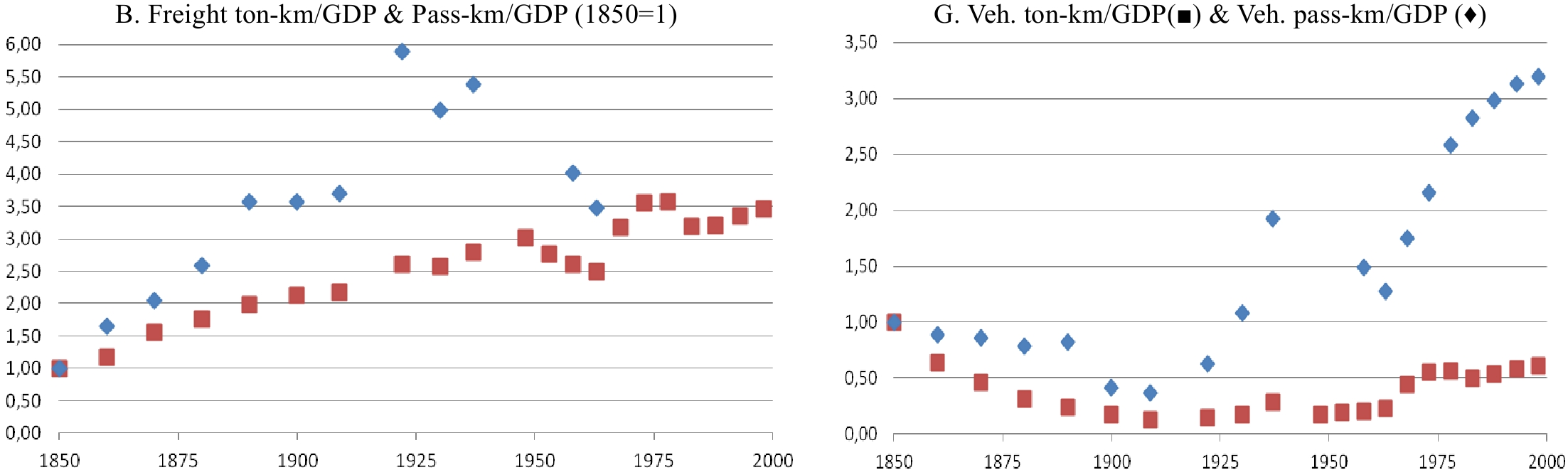
Figure 13. 

Road flow and vehicle intensities of GDP (ton-km & pass-km), France 1845−2005. Source: Gaudry^[24] (Fig. 2, p. 6), where the transformation from flows in B to vehicles in G is described in detail.

Vehicle traffic intensity of GDP and traffic density (congestion) could then be basic trends of opposite signs and with joint effects independent from any hypothetically lower rates of occupancy of vehicles or from better driver-vehicle-way interactions. In France the period 1845−1900 would have seen lower I (with some spurts) and decreasing congestion but the period 1910−2010 lower I (except for special sub-periods spurts) and increasing congestion. I is an imperfect substitute for the Total to Final output ratio.

Opposite effects of economic development on road safety

Two distinct features of economic development are conceivably also at work. First, increases in real GDP imply a slowly increasing share of services which gradually reduces the relative need for intermediate and predominantly physical supply chains and their intermediate transport flows; second, the ratio of Intermediate or Total (intermediate and final) to Final output can shift this base trend up or down, creating periods of trend reversal or acceleration. In all 18 OECD countries of Fig. 6, the accelerated diffusion of private car ownership after 1970 contributed to a higher share of services in final demand despite a general slowdown in public road building investments after 1967 ̶ as Intermediate output was also booming.

A tentative story of hewers of wood or coal and drawers of water

It is then possible to make some tentative sense of seemingly erratic secular series on the transport intensity of GDP and on its road traffic intensity I in particular, the latter fluctuating partly with vehicle capacity and with the intermediate to total output ratio of the Economy? Consider a development story.

Once upon a time, discretionary personal travel (i.e. visiting friends and relatives, trips to second homes, tourism) did not exist, except perhaps for the extremely rich. All travel could then be deemed 'essential', either to go to work or to market places (a final transport demand, in national accounts) or as part of work itself to produce the transport flows (an intermediate transport demand in input-output analysis) needed for inter-firm or inter-sector trade operations. Supply chains were predominantly physical (with human life often 'short and brutish') because the share of services or dematerialized consumption in final output was low, but increasing very slowly with development based on industrialization and with accompanying urbanization, both gradually emptying farms.

In 1845 France, for instance, it was frequent for people living in a part of town seldom to go for instance downtown, or never to visit even their own attractive national capital city, be it Paris. Life was all low-paid work without leisure and all travel (notably occupational) was dangerous, as measured by indices of fatalities per unit of distance travelled ̶ by any mode and by all modes. From this low GDP per capita base, growth required a relatively large quantity of material input which generated relatively high derived intermediate input and transport demand, causing the ratio of Intermediate to Total output to increase until about 1900 (as implied in Part A of Fig. 5 and shown in Fig. 13b) when a major turn occurred, just before the automobile regenerated, if it did not invent, personal travel.

Industrialization itself implied higher Intermediate to Total output, a higher I under constant modal shares and effects on economic inequality^[92]. But, during the last 150 years, there were significant ups and downs in the actual ratio of Intermediate to Total output, and consequently in I. To be less tentative would require more historical data on output, modes, flows, traffic and congestion.

We have developed, within the framework of aggregate yearly road safety models, a new explanation of the extraordinary occurrence in OECD countries of 18 national road fatality maxima clustered during the 5-year period 1970−1974 (including 11 in 1972−1973), referred to as 'The Matterhorn', a new name for the 1997 'The mystery of 1972−1973'^[47].

We have claimed that, in the long years since that diagnostic was made, no convincing explanation has been proposed of the existence of such national maxima in general and of their joint occurrence in particular. This despite significant research of common causes (e.g. congestion, baby boomer drivers' wave, new speed limits, new belt use laws, etc.) and despite resort to dodges (such as sigmoid time trends, splines and strict or flexible quadratic forms) imposed to induce a turning point of road safety performance, especially of fatalities. Such artificially forced turns were often based on GDP per capita but also on other variables such as the inverse of Smeed's vehicle availability (N/Population) interpreted as a vehicle occupancy rate. Complementarily, in the absence of a clear culprit or of 'a good idea' concerning the reasons for maxima and their clustering, it has also been much more difficult to explain the downward trends themselves, or the stagnations, in yearly national fatality and injury tallies expressed absolutely or as rates normalized by population or vehicle use.

Basic input-output economics and transport flows

As proposed recently^[45,93,94], we have accounted for The Matterhorn by enriching with I, Road traffic intensity of GDP, a representative aggregate model using Gross Domestic Product (GDP) per capita as key determinant of road accident and victim levels. Defined as road vehicle-kilometers per unit of constant GDP, I has stood as proxy for the relative level of total to final activity in The Economy. Indeed, because its numerator reflects transport demand for all economic activities, intermediate and final, which have long successfully intervened in a number of monthly road safety models, I can mimic natural up-and-down variations in total (intermediate and final) to final output, at least during our special spurt of clustered fatality peaks.

The usefulness of road safety outcome decompositions

We have explained both the presence of road fatality maxima in a number of countries (and to some extent of maxima in injuries, simultaneous with those of fatalities in the majority of cases) and their clustering in OECD countries between 1970 and 1974 using a representative yearly DRAG-type decomposition with total bodily injury accidents (the sum of fatal and not fatal occurrences), their severity rates per accident (morbidity and mortality), and their victims by category (injured, killed). This has revealed effects differentiated by dimension.

An economic spine in lieu of splines

The gains resulting from the addition of the new naturally turning variable I have been spectacular and have led us to expect that various forms of transport intensity of GDP might contribute to the explanation of other peaks in transport fatalities, for instance that of air victims which occurred also in 1972−1974^[95] and may have been partially caused by a related spurt in air traffic intensity of GDP. For countries where road fatalities have yet to peak, the next analytical safety work task is that of forecasting the profile of Intermediate to Final output in the economy of the country; it is not to collect guesses by local road safety experts on the future long-term evolution of current local indicator trends.

Road traffic intensity of GDP has a multi-secular history

We have also distinguished between I during The Matterhorn sub-period and during the last 175 years of variations associated with industrialization and urbanization. As Matterhorn lustrum times run counter to a downward trend in the Fatality intensity of road traffic observable since 1910 in France and the USA, we have proposed a tentative conceptual list of checkpoints, based on known secular trends, for determining whether the I proxy might make sense in another yearly road safety model tailored to a particular historical sub-period, such as the post-Great Depression spurt in the USA.

Glorious but gory

Overall, we noted that rising intermediate output brings out the 'bloody mathematics of our condition', as written in 1942 by Albert Camus, who died in a 1960 car accident. We have indirectly shown it to be relevant to our time of de-industrialization and delocalization of manufacturing to less economically developed countries. This no doubt also displaces many of the road safety and other negative externalities incurred by those who were there before and for whom the recent Golden 30 years of economic growth (1945−1975) were perhaps not all glory after all. This new emphasis on the link between intermediate economic output and road safety strengthens the backbone of current management of yearly safety indicators and trends, and not only in countries that have yet to see a global maximum of their fatalities.