-
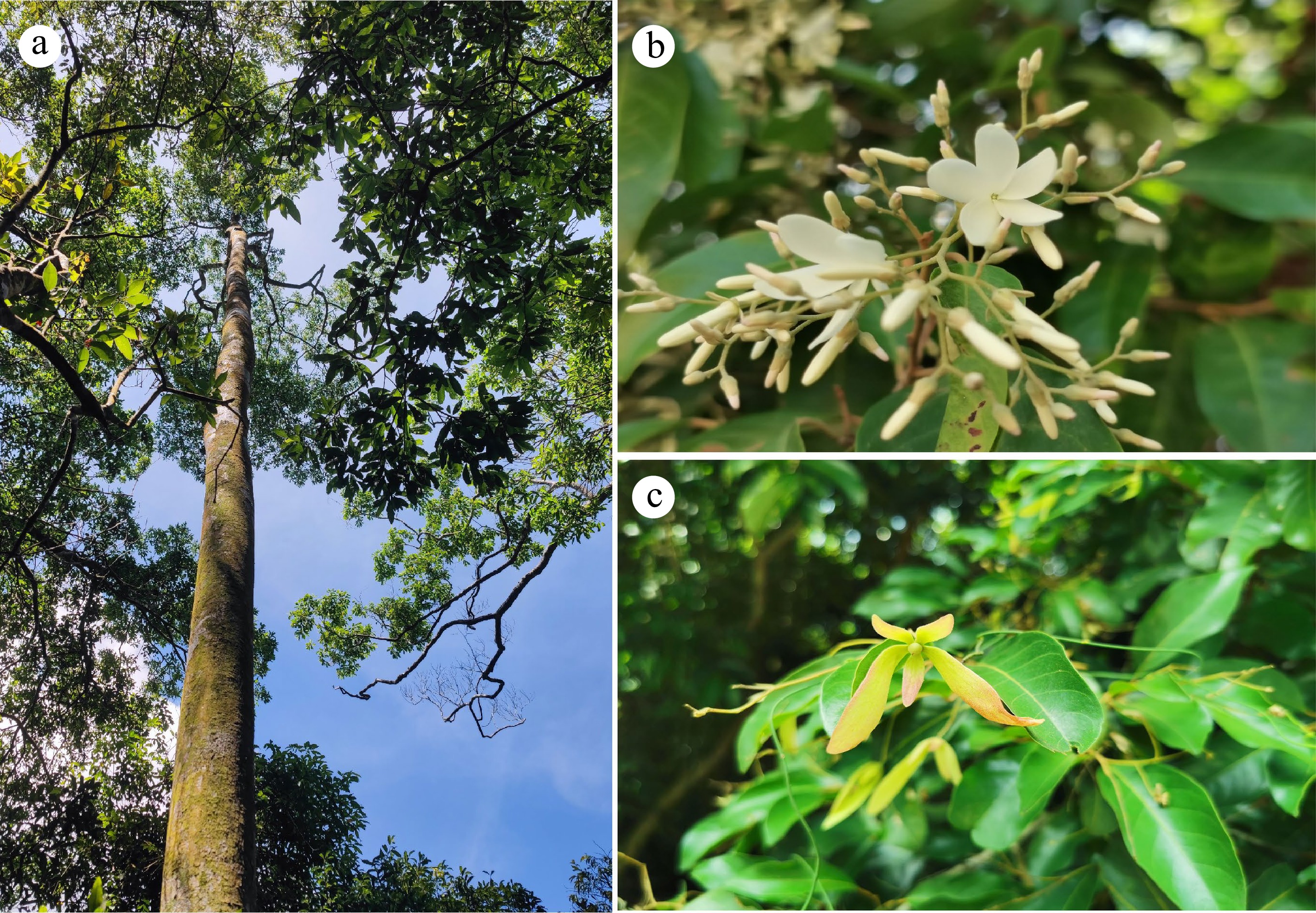
Figure 1.
Morphology of Vatica mangachapoi. (a) An individual tree, (b) flowers, (c) fruits.
-
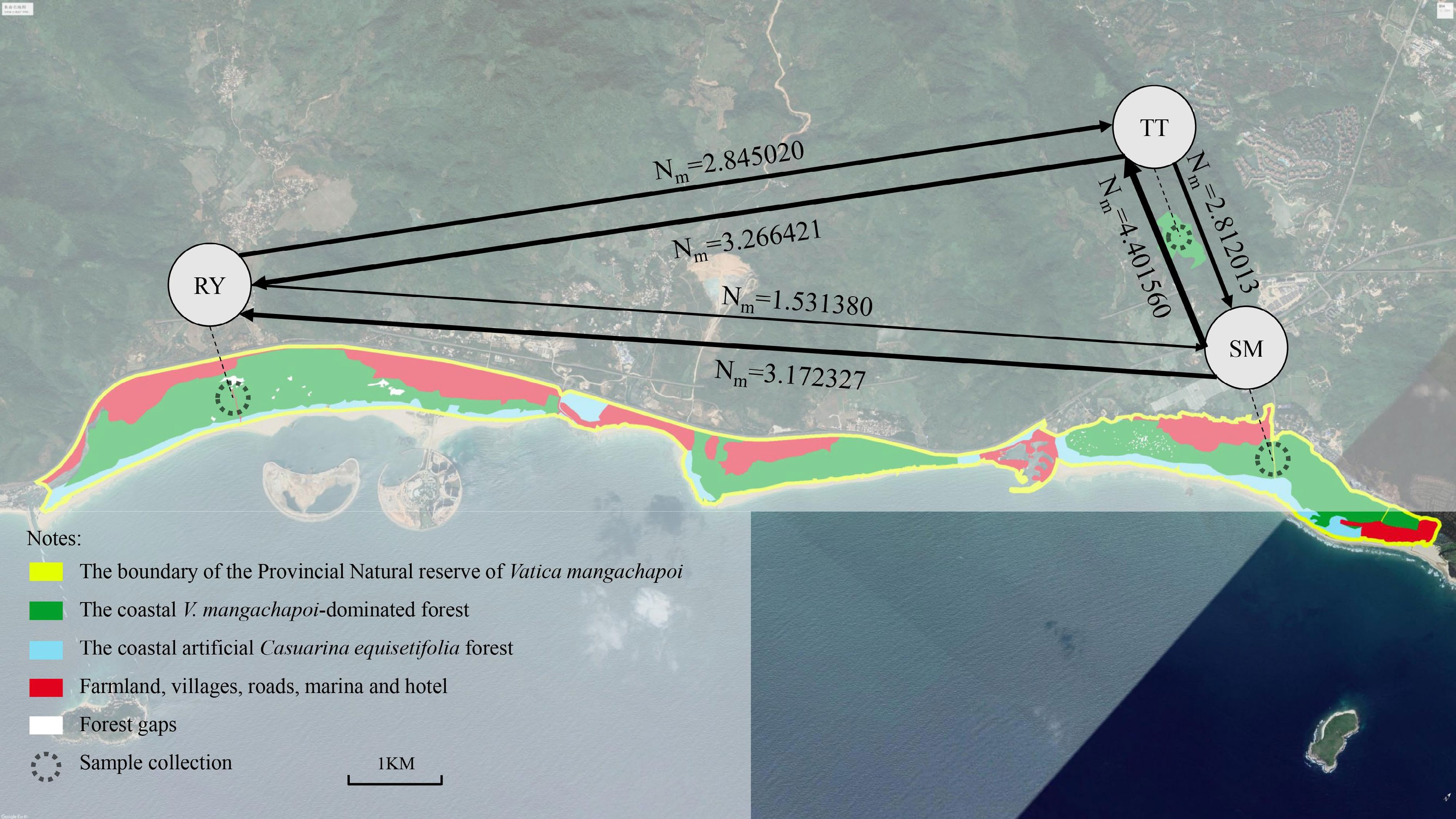
Figure 2.
Geographic distribution of the coastal V. mangachapoi-dominated forest and the locations of the three sampled V. mangachapoi populations. Gene flow among them was estimated, with the width of lines being proportional to the intensity of gene flow.
-
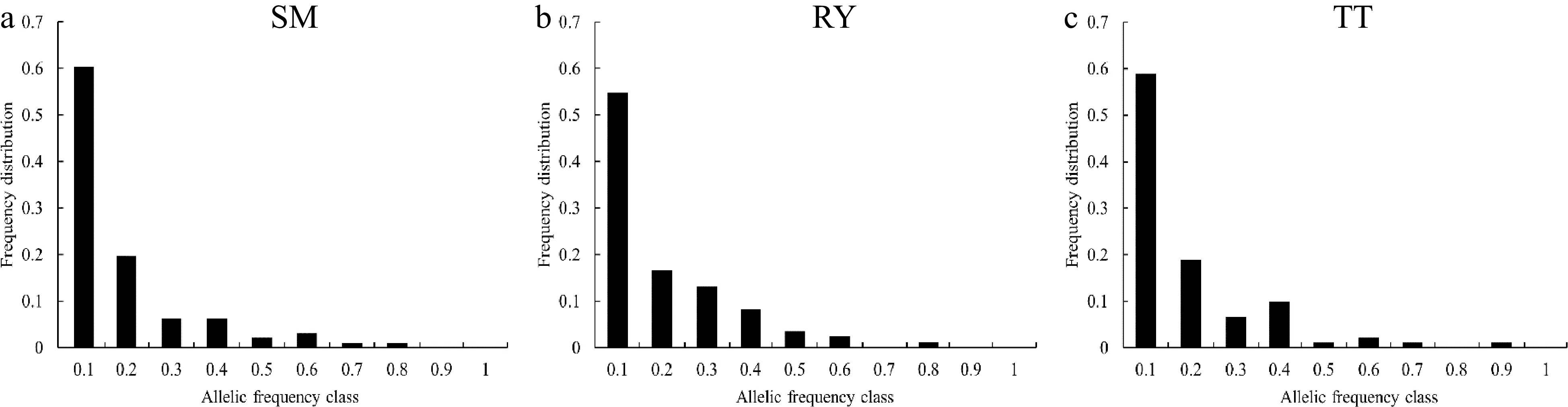
Figure 3.
Allele frequency distribution of the three V. mangachapoi populations.
-
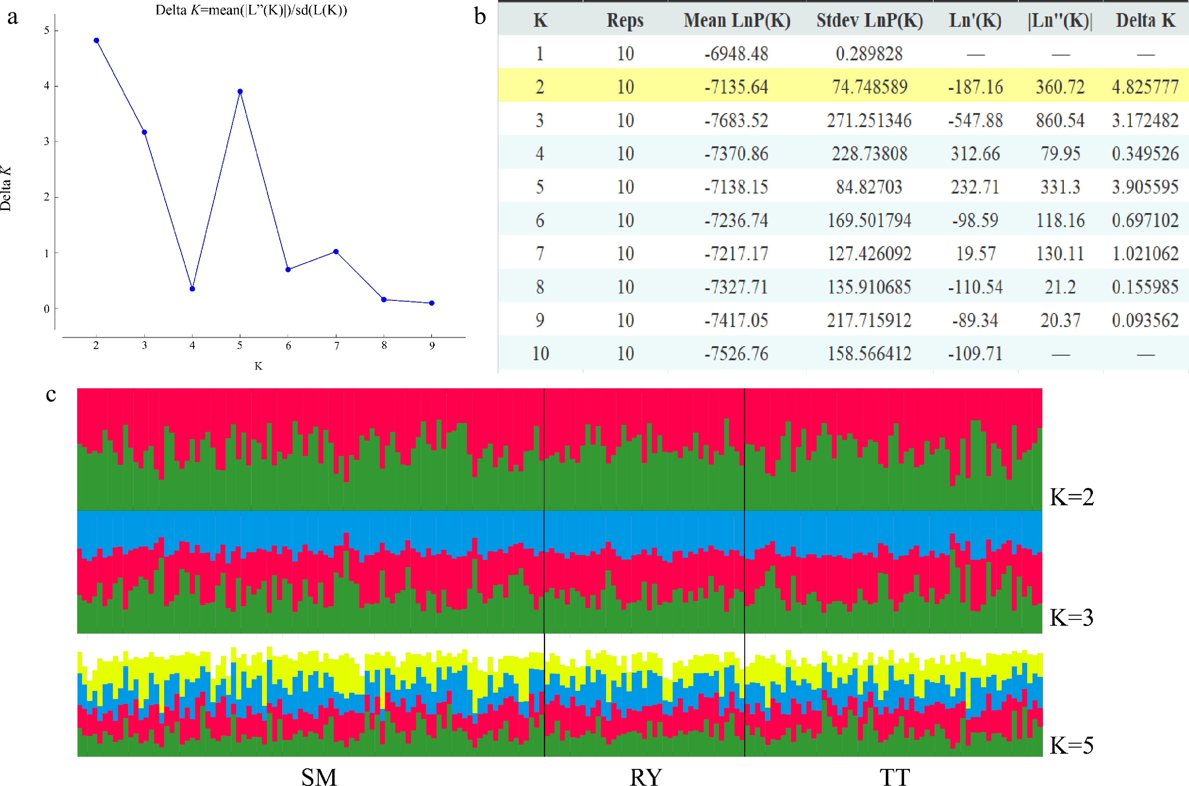
Figure 4.
Results of STRUCTURE analysis. (a) Best K determined using the delta K method. (b) Log probabilities and delta K values for K from two to ten. (c) The results of individual assignment at K = 2, 3 and 5. Each vertical bar represents an individual, and the proportion of the colors corresponds to the posterior probability of genetic clusters assigned to each individual.
-
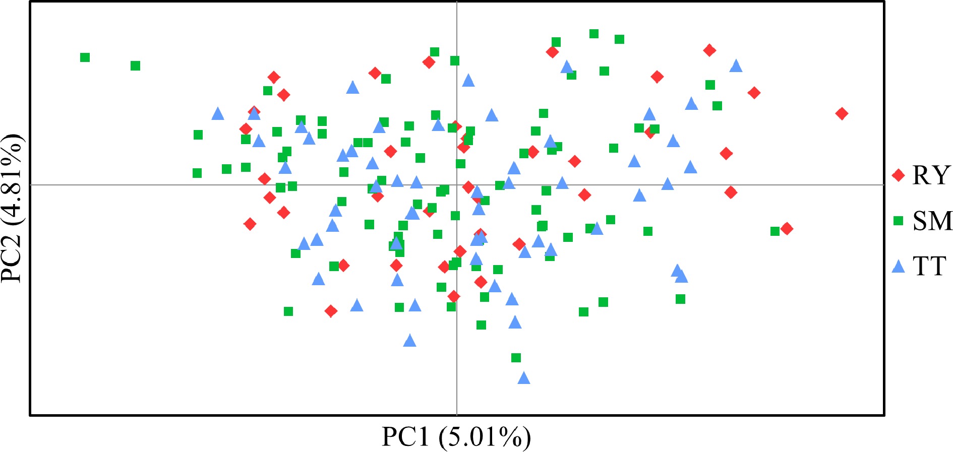
Figure 5.
Principal co-ordinate analysis (PCoA) based on Nei & Chessers[30] genetic distance among individual samples of V. mangachapoi.
-
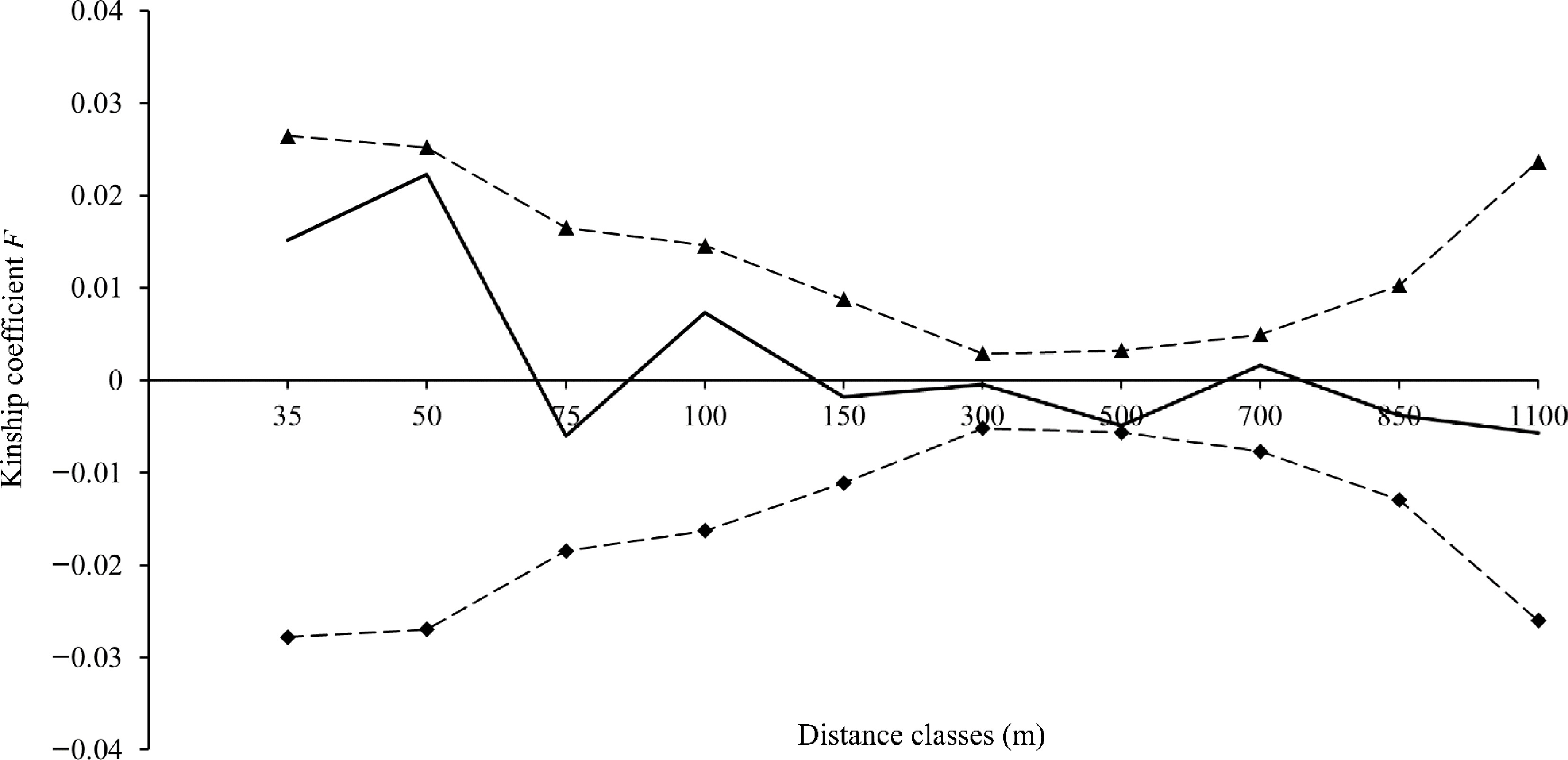
Figure 6.
Fine-scale genetic structure of V. mangachapoi in Shimei Bay. The solid line represents the mean Kinship coefficient F (Loiselle et al.[41]), and the dashed lines represent the 95% confidence intervals of the mean Kinship coefficient F.
-
Population Location N Na Ne Ho He Fis SM 110.26691° E, 18.66671° N 91 8 3.647 0.547 0.690 0.207 RY 110.17952° E, 18.59768° N 39 7 3.704 0.605 0.700 0.142 TT 110.24941° E, 18.67744° N 58 7.5 3.694 0.566 0.692 0.167 Average 7.5 3.682 0.572 0.694 0.172 Table 1.
Genetic diversity indices of the three V. mangachapoi populations based on 12 SSR markers.
-
Loci Primer sequences (5’-3’) Repeat
motifAllele size GenAlex PowerMarker Na Ne Ho He PIC VM1 F:GAACCCTTATTGGCCTGCCTAC (AT)11 166−184 7.333 4.231 0.740 0.763 0.7430 R:GGGACCAAATGACTTGAGTAATCT VM2 F:ACCCTAACAATTCTCTTTGTTTCCT (TAA)11 152−195 9.667 4.120 0.513 0.755 0.7364 R:CCCCAATCTCAGTAAGGACTCA VM3 F:CTTGTGTCGAGCATGCATGTAT (AT)11 175−191 8.333 4.857 0.761 0.793 0.7659 R:TGCTGGCCTTTTATGTTAGGGT VM4 F:ATAGCAGGCACTTCGGAAGTAC (TA)8 261−277 8.667 4.613 0.370 0.781 0.7533 R:CCTGAGAAACAAAGCAACGCAT VM5 F:GCACTAGCACTAGCACTAGCTT (CT)11 218−226 4.667 2.908 0.629 0.651 0.6026 R:GGCTTTTCCAATTTCCATGGCT VM6 F:AGTTAAGGGACCAAATTTAGCGT (TA)7 259−269 5.000 2.794 0.593 0.636 0.5902 R:GTGTTTGTCAACTGGGCTTCAA VM7 F:CCCATGTGCTAGGCTAATGCTA (AT)6 229−239 5.000 2.394 0.303 0.582 0.5409 R:AAATCAGCATGAAACTTCTCCATT VM8 F:CACCACCACAGGCTTGAGTATA (TA)7 168−182 5.667 1.722 0.374 0.415 0.4044 R:GAAGGCCAACTAATCAAGCTGC VM9 F:TCATTTCTGTCTCACTCGACCC (TTC)10 148−168 5.667 3.010 0.639 0.666 0.6097 R:TCATCGACGAATCACTGTTCGA VM10 F:ACGGATAAGTTAACGGACTAGACA (TA)10 215−227 9.333 4.713 0.568 0.776 0.7997 R:AGATTTTCCCCCAGTCATCGAC VM11 F:GCTGGCACTTAGGATGCCTTAA (ATT)11 138−150 11.000 3.564 0.610 0.702 0.6657 R:AGCAACCAATTAGCTCAAATCAA VM12 F:GGGCAGCCTCGTAAATCAATTAC (ATT)13 225−249 9.667 5.253 0.769 0.808 0.7958 R:ATTACCTGGCACAACCTTAGCC Table 2.
Primer sequences, allele size and genetic diversity indices of the 12 SSR markers.
-
Direction of
gene flowMigration
rate (M)Effective population
size (θ)Gene flow (Nm) SM→RY 129.615 θSM = 0.09790 3.172327 SM→TT 179.839 4.401560 RY→SM 63.241 θRY = 0.09686 1.531380 RY→TT 117.490 2.845020 TT→SM 115.412 θTT = 0.09746 2.812013 TT→RY 134.062 3.266421 Table 3.
Mutation-scaled migration rate, effective population size and gene flow estimated by program MIGRATE.
Figures
(6)
Tables
(3)