-
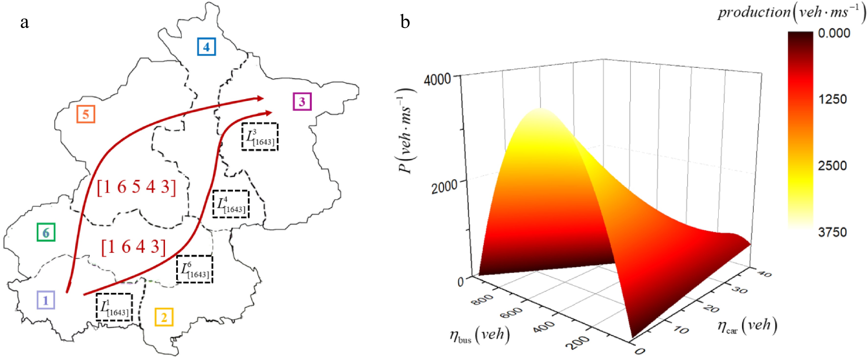
Figure 1.
A multi-reservoir network. (a) Network partitioning and characteristics. (b) 3D-MFD surface which the formula refers to Paipuri & Leclercq[27].
-
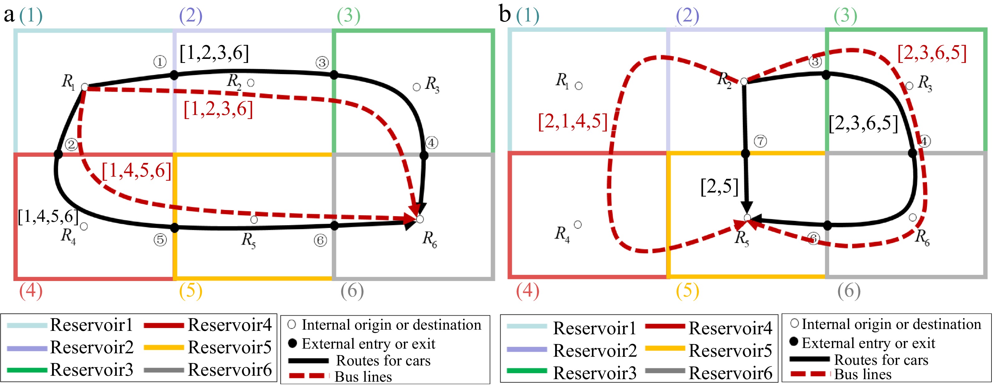
Figure 2.
Reservoir system configuration. (a) The regional OD pair (1−6). (b) The regional OD pair (2−5).
-
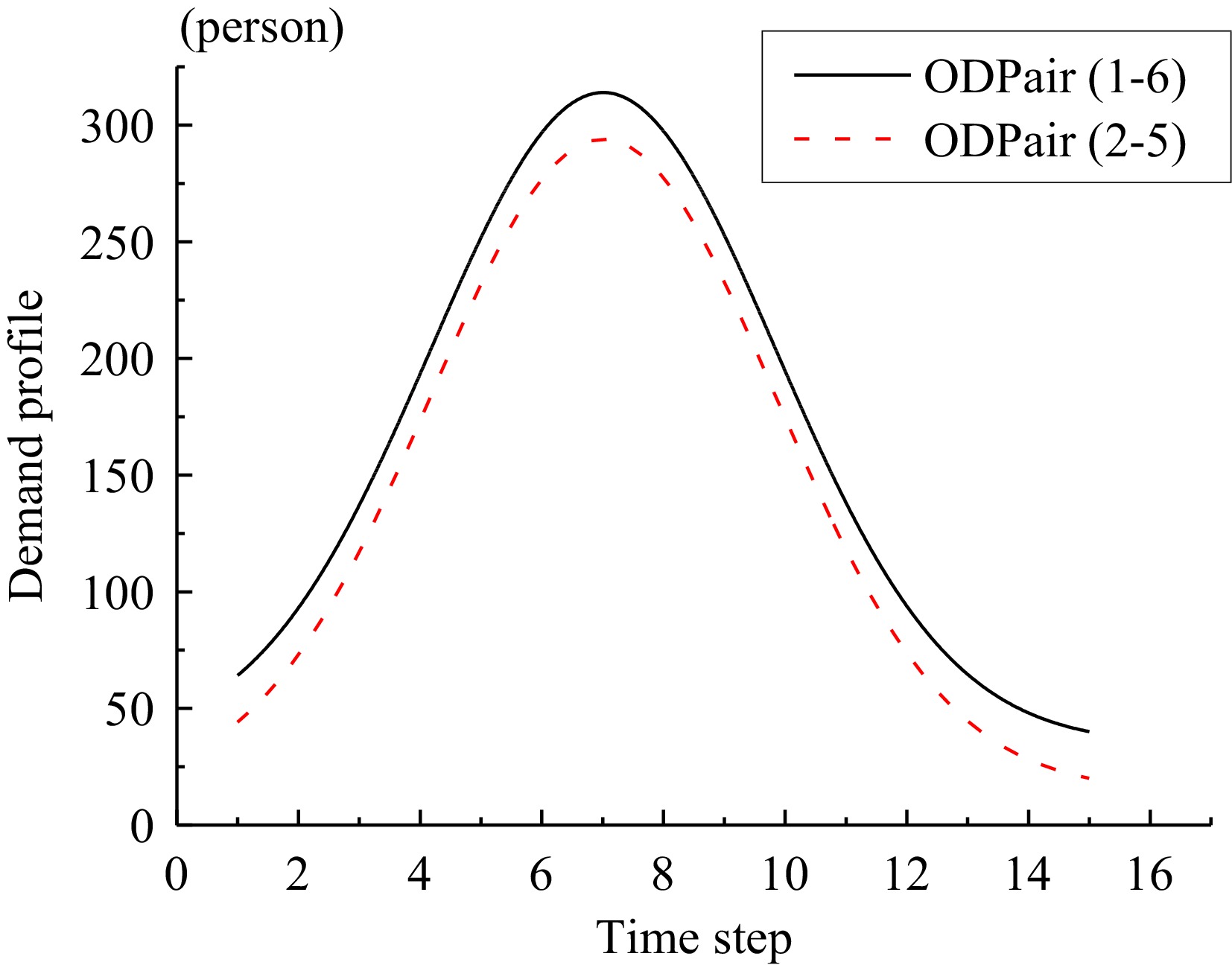
Figure 3.
OD demand profile.
-
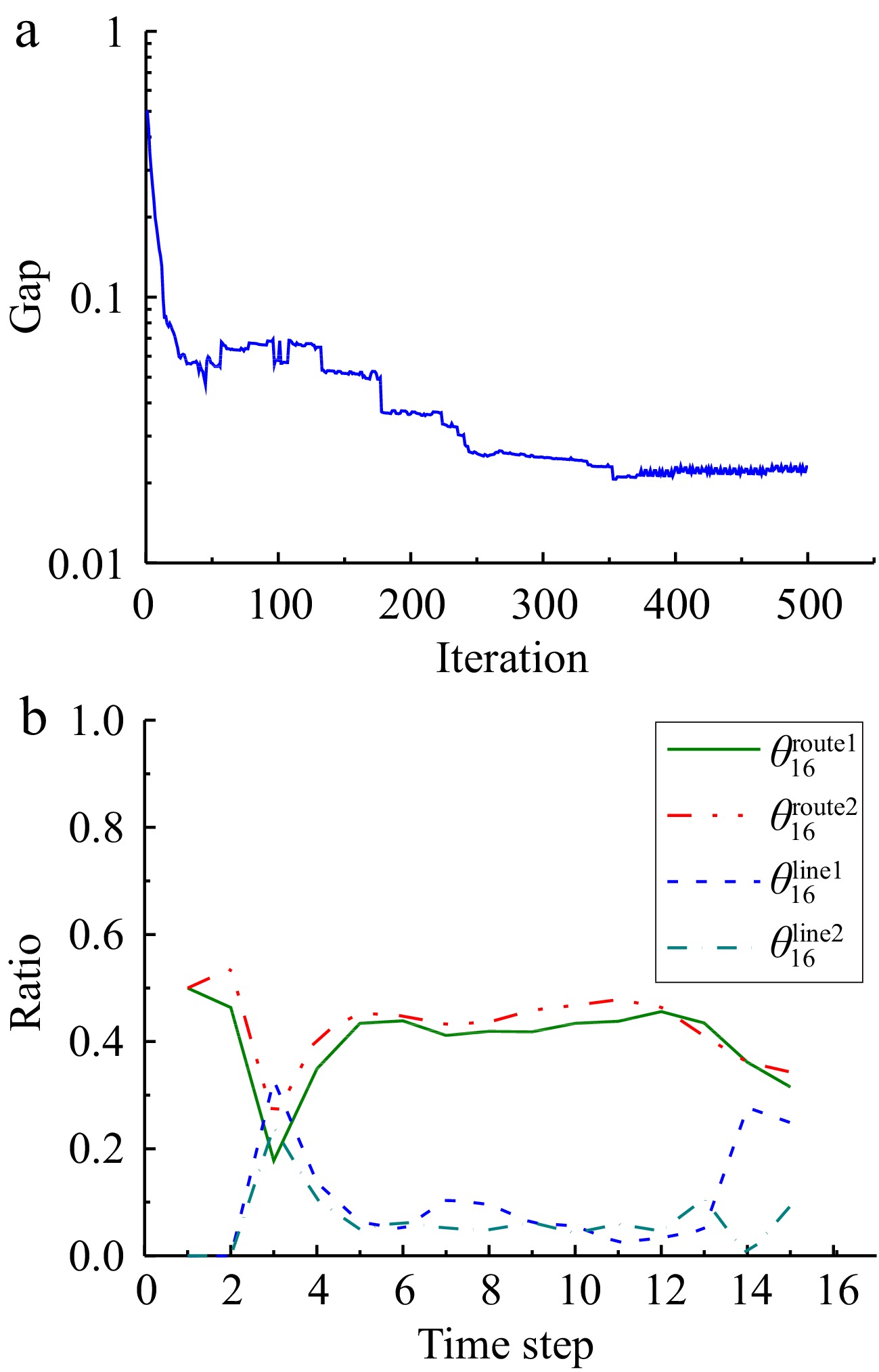
Figure 4.
Results using double projection algorithm. (a) Convergence of double projection algorithm. (b) Route choice parameters for an OD pair.
-
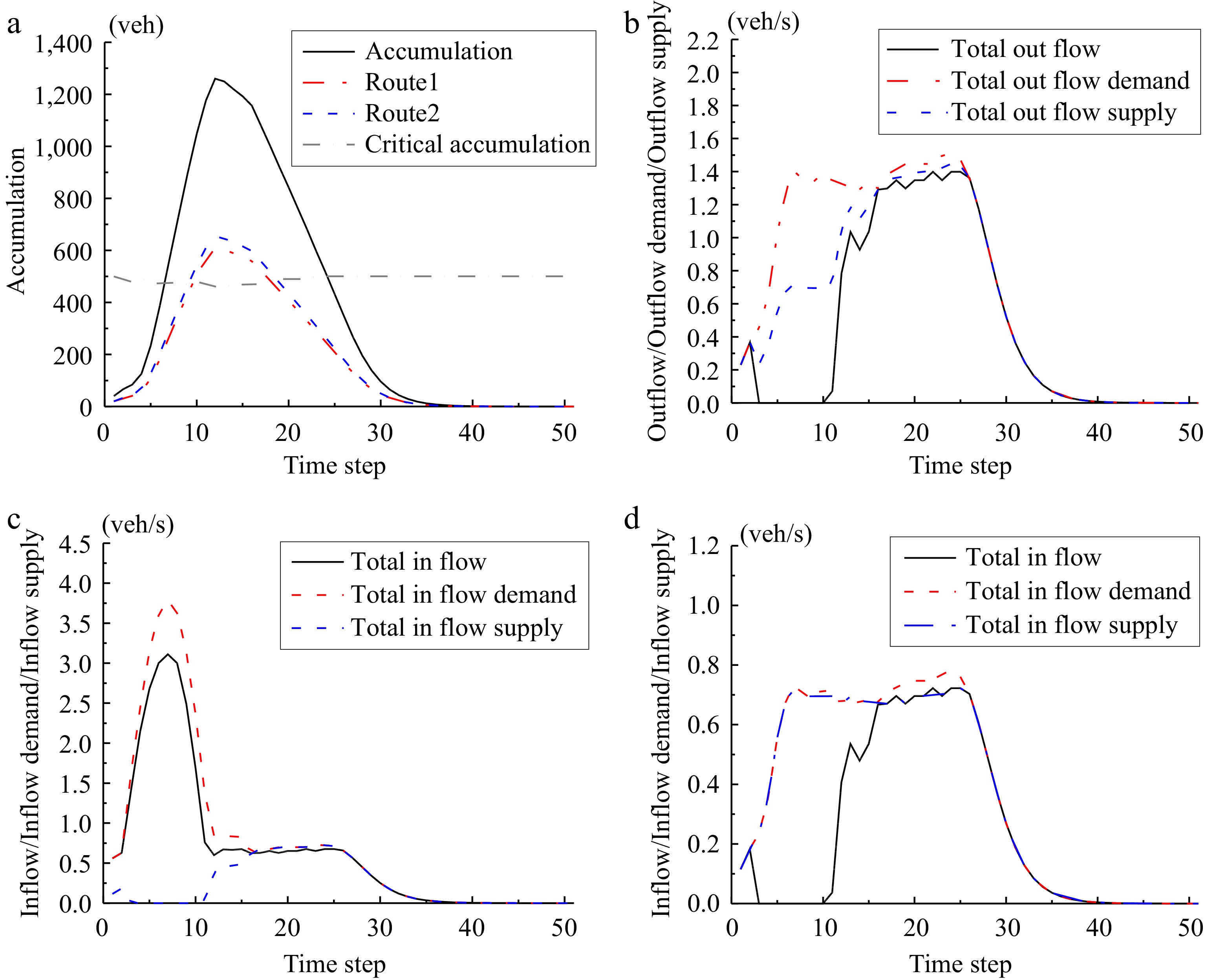
Figure 5.
Traffic dynamics. (a) Evolution of car accumulation in Reservoir 1. (b) Evolution of outflow in Reservoir 1. (c) Evolution of inflow in Reservoir 2. (d) Evolution of inflow in Reservoir 4.
-
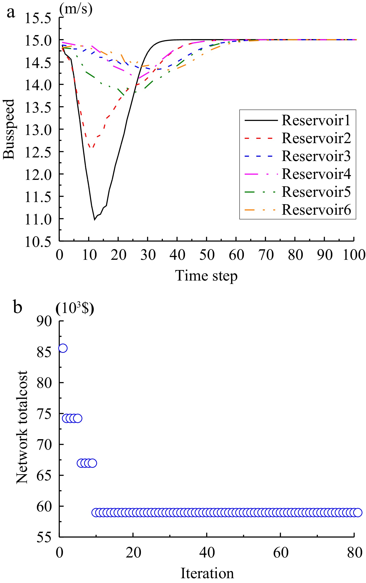
Figure 6.
Results on the (a) bus speed evolution and (b) convergence of the surrogate model based algorithm.
-
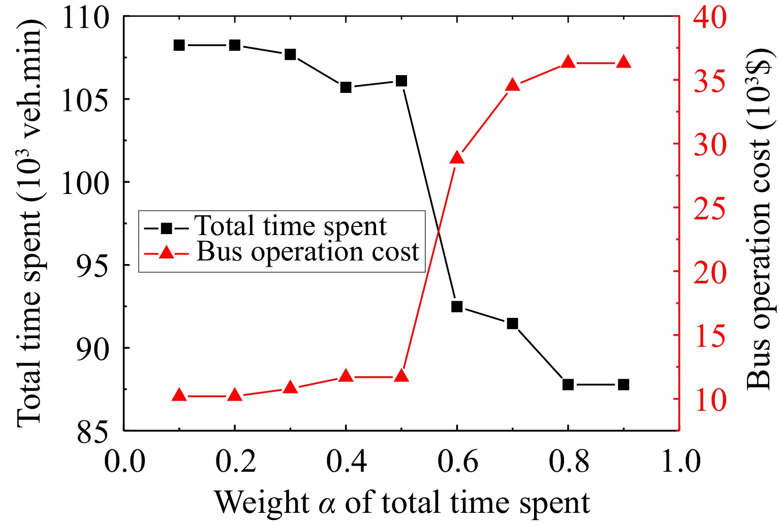
Figure 7.
Changes in the total time spent and bus operation cost for different weight values (α).
-
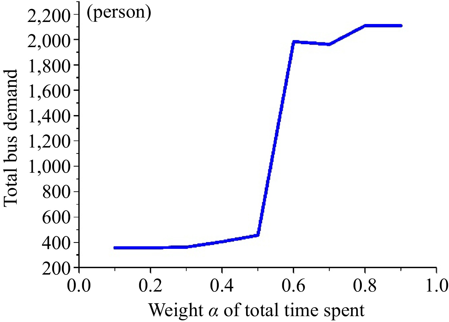
Figure 8.
The influence of the total time spent on the demand for bus travel.
-
Input: Reservoir initial bus accumulation $\eta _{{\text{p,r}}}^{{\text{bus}}}\left( {{t_0}} \right)$ $\eta _{{\text{p,r}}}^{{\text{car}}}\left( {{t_0}} \right)$ $L_{{\text{p,r,t}}}^{{\text{bus}}}\left( {{t_{\text{0}}}} \right){\text{ = 0}}$ $t$ $t$ $\lambda _{\text{p}}^{{\text{w,bus}}}\left( t \right)$ $T$ $\delta t$ 1: for $t = {t_0}$ ${t_0} + T$ $\delta t$ 2: According to the bus and car accumulation which is calculated by Eq. (1), combined with reservoir 3D-MFD, the bus speed $v_{\text{r}}^{{\text{bus}}}\left( t \right)$ 3: for $r = 1$ $N$ 4: Inflow: if $r = o$ $\eta _{{\text{p,r,in}}}^{{\text{bus}}}\left( t \right) = \lambda _{\text{p}}^{{\text{w,bus}}}\left( t \right) \cdot \delta t$ $\eta _{{\text{p,r,in}}}^{{\text{bus}}}\left( t \right) = \eta _{{\text{p,}}{{\text{p}}^{\text{ - }}}\left( {\text{r}} \right){\text{,out}}}^{{\text{bus}}}\left( t \right)$ 5: Outflow: track the trip distance $L_{{\text{p,r,t}}}^{{\text{bus}}}\left( {t{\text{ + }}\delta t} \right) = L_{{\text{p,r,t}}}^{{\text{bus}}}\left( t \right) + v_{\text{r}}^{{\text{bus}}}\left( t \right) \cdot \delta t$ 6: if $L_{{\text{p,r,t}}}^{{\text{bus}}}\left( {t{\text{ + }}\delta t} \right) > L_{{\text{p,r}}}^{{\text{bus}}}$ 7: if $r = d$ $ {\tau _{{\text{p,bus,travel}}}}\left( t \right) = {\tau _{{\text{p,bus,travel}}}}\left( t \right) + {t_{\text{s}}} $ $\eta _{{\text{p,r,out}}}^{{\text{bus}}}\left( t \right) = \eta _{{\text{p,r,in}}}^{{\text{bus}}}\left( {t{\text{ - }}{\tau _{{\text{p,bus,travel}}}}\left( t \right)} \right)$
where${t_{\text{s}}}$ $r$ 8: else ${\tau _{{\text{p,bus,travel}}}}\left( t \right) = {\tau _{{\text{p,bus,travel}}}}\left( t \right) + \delta t$ $\eta _{{\text{p,r,out}}}^{{\text{bus}}}\left( t \right) = \eta _{{\text{p,r,in}}}^{{\text{bus}}}\left( {t{\text{ - }}{\tau _{{\text{p,bus,travel}}}}\left( t \right)} \right)$ 9: else ${\tau _{{\text{p,bus,travel}}}}\left( t \right) = {\tau _{{\text{p,bus,travel}}}}\left( t \right) + \delta t$ $\eta _{{\text{p,r,out}}}^{{\text{bus}}}\left( t \right) = 0$ 10: Bus accumulation update: $\eta _{{\text{p,r}}}^{{\text{bus}}}\left( {t + \delta t} \right) = \eta _{{\text{p,r}}}^{{\text{bus}}}\left( t \right) + \eta _{{\text{p,r,in}}}^{{\text{bus}}}\left( t \right) - \eta _{{\text{p,r,out}}}^{{\text{bus}}}\left( t \right)$ 11: end for 12: end for Output: reservoir bus accumulation $\eta _{{\text{p,r}}}^{{\text{bus}}}\left( t \right)$ ${\tau _{{\text{p,bus,travel}}}}\left( t \right)$ Table 1.
Trip-based solver algorithm.
-
Input: projection step $\bar \rho $ $\varepsilon > 0$ $\beta $ $ \xi \in \left(\text{0},\text{1}\right) $ ${P^{\text{w}}}$ 1: Initial path demand ${{\mathbf{f}}^0}\left( k \right) = {\lambda ^{\text{w}}}\left( k \right)/\varsigma $ $\varsigma $ $w$
time${\mathbf{\tau }}$ ${\rho ^0} = \bar \rho $ $\gamma = 0$ 2: while $G({{\mathbf{f}}^{\text{γ }}}) > \varepsilon $ 3: Compute ${{\mathbf{\bar f}}^{\text{γ }}}(k) = {\text{pro}}{{\text{j}}_\Omega }({{\mathbf{f}}^{\text{γ }}}(k) - {\rho ^{\text{γ }}}{\mathbf{\tau }}({{\mathbf{f}}^{\text{γ }}}(k)))$ 4: while ${\rho ^{\text{γ }}} > \beta \frac{{\left\| {{{\mathbf{f}}^{\text{γ }}}(k) - {{{\mathbf{\bar f}}}^{\text{γ }}}(k)} \right\|}}{{\left\| {{\mathbf{\tau }}({{\mathbf{f}}^{\text{γ }}}(k)) - {\mathbf{\tau }}({{{\mathbf{\bar f}}}^{\text{γ }}}(k))} \right\|}}$ 5: ${\rho ^{\text{γ }}} = \min \left\{ {\xi {\rho ^{\text{γ }}},\beta \frac{{\left\| {{{\mathbf{f}}^{\text{γ }}}(k) - {{{\mathbf{\bar f}}}^{\text{γ }}}(k)} \right\|}}{{\left\| {{\mathbf{\tau }}({{\mathbf{f}}^{\text{γ }}}(k)) - {\mathbf{\tau }}({{{\mathbf{\bar f}}}^{\text{γ }}}(k))} \right\|}}} \right\}$ 6: Compute ${{\mathbf{\bar f}}^{\text{γ }}}(k) = {\text{pro}}{{\text{j}}_\Omega }({{\mathbf{f}}^{\text{γ }}}(k) - {\rho ^{\text{γ }}}{\mathbf{\tau }}({{\mathbf{f}}^{\text{γ }}}(k)))$ 7: end while 8: Compute ${{\mathbf{f}}^{{\text{γ + 1}}}}(k) = {\text{pro}}{{\text{j}}_\Omega }({{\mathbf{f}}^{\text{γ }}}(k) - {\rho ^{\text{γ }}}{\mathbf{\tau }}({{\mathbf{\bar f}}^{\text{γ }}}(k)))$ 9: Update travel time vector ${\mathbf{\tau }}({{\mathbf{f}}^{\gamma + 1}}(k))$ $\gamma = \gamma + 1$ 10: end while Output: flow vector ${{\mathbf{f}}^{\text{γ }}}(k)$ Table 2.
Double projection algorithm.
-
Input: the maximum iterations ${\gamma _{\max }}$ $ C_{{\text{success}}}^{{\text{max}}} $ $ C_{{\text{fail}}}^{{\text{max}}} $ $ p_{{\text{slct}}}^{{\text{init}}} $ 1: Initialization 1.1 initial evaluation points set. ${I_0} = \left\{ {{{\mathbf{y}}_1},{{\mathbf{y}}_2}, \ldots ,{{\mathbf{y}}_{{{\text{n}}_{\text{0}}}}}} \right\}$ ${n_0}$ ${\mathbf{Z}} = \left[ {Z\left( {{{\mathbf{y}}_{\text{i}}}} \right),{{\mathbf{y}}_{\text{i}}} \in {I_0}} \right]$ ${{\mathbf{y}}_{\text{i}}} = \left\{ {{{\left\{ {{f_1},{f_2}, \ldots ,{f_{{{\text{n}}_{\text{0}}}}}} \right\}}^{\text{i}}}} \right\}$ $Z\left( {{{\mathbf{y}}_{\text{i}}}} \right)$ ${{\mathbf{y}}_{{\text{best}}}}$ $\gamma = 0$ 1.2 initialization parameters. Initialize the counters of consecutive successes ${C_{{\text{sucess}}}} = 0$ ${C_{{\text{fail}}}} = 0$ $C_{{\text{success}}}^{\max }$ $C_{{\text{fail}}}^{{\text{max}}}$ $p_{{\text{slct}}}^{\text{0}} = p_{{\text{slct}}}^{{\text{init}}}$ 2: Repeat 3: Update surrogate model.
Use the evaluation point set${I_{\text{n}}}$ ${\prod _{\text{n}}} = \left\{ {\left( {{{\mathbf{y}}_{\text{i}}},Z\left( {{{\mathbf{y}}_{\text{i}}}} \right)} \right),{{\mathbf{y}}_{\text{i}}} \in {I_{\text{n}}}} \right\}$ ${S_{\text{n}}}\left( {\mathbf{y}} \right)$ 4: Candidate points set generation.
Based on the perturbation probability$ {p_{{\text{slc}}t}} $ ${E_{\text{n}}}$ ${{\mathbf{y}}_{{\text{best}}}}$ 5: Select the evaluation point.
Each candidate point is scored. Set${{\mathbf{y}}_{{\text{n+1}}}}$ $Z({{\mathbf{y}}_{{\text{n+1}}}})$ 7: Update the optimal solution.
If$Z({{\mathbf{y}}_{{\text{n+1}}}}) < Z({{\mathbf{y}}_{{\text{best}}}})$ ${{\mathbf{y}}_{{\text{best}}}} = {{\mathbf{y}}_{{\text{n+1}}}}$ $Z({{\mathbf{y}}_{{\text{best}}}}){\text{ = }}Z({{\mathbf{y}}_{{\text{n+1}}}})$ ${C_{{\text{success}}}} = {C_{{\text{success}}}} + 1$ ${C_{{\text{fail}}}} = 0$ ${C_{{\text{fail}}}} = {C_{{\text{fail}}}} + 1$ ${C_{{\text{success}}}} = 0$ 8: Adjust disturbance probability.
If$ {C_{{\text{success}}}} > C_{{\text{success}}}^{{\text{max}}} $ $ p_{{\text{slct}}}^{{\text{n+1}}} = \min \{ 2p_{{\text{slct}}}^{\text{n}},p_{{\text{slct}}}^{{\text{max}}}\} $ $ {C_{{\text{success}}}} = 0 $
If$ {C_{{\text{fail}}}} > C_{{\text{fail}}}^{{\text{max}}} $ $ p_{{\text{slct}}}^{{\text{n+1}}} = \max \{ p_{{\text{slct}}}^{\text{n}}/2,p_{{\text{slct}}}^{{\text{min}}}\} $ $ {C_{{\text{fail}}}} = 0 $ $\gamma = \gamma + 1$ 9: Update the evaluation points set. ${I_{{\text{n+1}}}} = {I_{\text{n}}} \cup \{ {{\mathbf{y}}_{{\text{n+1}}}}\} $ 10: Until $\gamma \geqslant {\gamma _{\max }}$ Output: ${{\mathbf{y}}_{{\text{best}}}}$ Table 3.
Surrogate model-based algorithm.
-
Characteristics [units] ${R_1}$ ${R_2}$ ${R_3}$ ${R_4}$ ${R_5}$ ${R_6}$ Trip length $L_{\text{1}}^{{\text{car}}}$ [m] 2500 5000 5000 − − 2500 Trip length $L_{\text{2}}^{{\text{car}}}$ [m] 2500 − − 5000 5000 2500 Trip length $L_3^{{\text{car}}}$ [m] − 2500 − − 2500 − Trip length $L_{\text{4}}^{{\text{car}}}$ [m] − 2500 5000 − 2500 5000 Bus line $L_{\text{1}}^{{\text{bus}}}$ [m] 2500 5000 5000 − − 2500 Bus line $L_{\text{2}}^{{\text{bus}}}$ [m] 2500 − − 5000 5000 3500 Bus line $L_{\text{3}}^{{\text{bus}}}$ [m] 5000 2500 − 5000 2500 − Bus line $L_{\text{4}}^{{\text{bus}}}$ [m] − 2500 5000 − 2500 5000 Table 1.
Reservoir characteristics, where
$L_{\text{1}}^{{\text{car}}}$ $L_{\text{2}}^{{\text{car}}}$ $L_3^{{\text{car}}}$ $L_{\text{4}}^{{\text{car}}}$ $L_{\text{1}}^{{\text{bus}}}$ $L_{\text{2}}^{{\text{bus}}}$ $L_{\text{3}}^{{\text{bus}}}$ $L_{\text{4}}^{{\text{bus}}}$ -
Simulation 3D-MFD 2D-MFD The optimal frequency (min) {3.0, 4.0, 4.0, 3.0} {4.0, 0.2, 2.0, 1.0} Total time spent (veh·min) 106088.75 93111.93 Operation cost ( ${\$}$ 11700 44400 The objective value ( ${\$}$ 58894.38 68755.96 Table 2.
Total travel time of passengers and operation cost using 3D-MFD and 2D-MFD respectively.
-
Simulation Equilibrium Non-equilibrium Total time spent (veh·min) 106088.75 177269.47 Operation cost (min) 11700 35400 The objective value $\left( {\$} \right)$ 58894.38 106334.73 Table 3.
The optimal solution under equilibrium and non-equilibrium type.
-
Simulation The optimal
frequency (min)The objective value ( $ {\$} $ $\Delta {Z_{\text{i} } }$ Scenario 1
(2D-MFD non-equilibrium){1.0, 0.5, 0.5, 0.5} 68,544.698 16.39 Scenario 2
(2D-MFD equilibrium){4.0, 0.2, 2.0, 1.0} 68,755.964 16.74 Scenario 3
(3D-MFD non-equilibrium){1.0, 0.5, 1.0, 1.0} 65,623.043 11.42 Scenario 4
(3D-MFD equilibrium){3.0, 4.0, 4.0, 3.0} 58,894.376 − Table 4.
Comparison of the results of the optimal solution in 4 scenarios.
Figures
(8)
Tables
(7)