


-
Public transport is a key component of a sustainable transport system. In many cities, public transport is considered as a promising solution to urban traffic congestion. A properly designed public transport system is expected to improve traffic efficiency by minimizing the total delays of citizens. In a multi-modal system, buses can take more passengers, while moving slower than private cars. A high-frequency bus service would decrease the average traffic speed and hence increase traffic delays, while a low-frequency bus service would increase the waiting time of passengers at bus stops. As argued in literature, the waiting time at bus stops is a key element in a passenger's assessment of bus service quality[1,2]. The bus service quality could affect the demand for each transport mode, e.g., buses and cars. Hence, the bus frequency can be optimized to minimize the total delays of the transport system, including the time spent by both bus passengers and car users. To optimize bus frequency, it is necessary to integrate the congestion dynamics and its impacts on the mode choices in the optimization formulation.
Optimizing bus frequency will help improve the bus service and alleviate traffic congestion, because a good bus service could reduce car demand. However, in most of the literature on bus frequency optimization, the demand is static[3−6]. The static demand ignores the interactions between buses and cars, and its impacts on travelers' mode choices. The static demand assumption rules out impacts of bus service on the demand elasticity.
The interaction between cars and buses would determine the travel speed and delays of each mode, which will finally shape the demand for each mode. To predict the mode choice, it is necessary to model the multi-modal congestion dynamics. However, the congestion dynamics in bus frequency optimization is frequently modeled by a Bureau of Public Roads (BPR) function. The BPR function is too simple to describe the multi-modal congestion dynamics. Some attempts[7,8] have considered multi-modal congestion dynamic when optimizing the public transport system. The interaction between cars and buses is described by a 3D-MFD based model. But the demand including a car demand and a public transport passenger demand, is given exogenously. That is, the impacts of traffic congestion and the bus system performance (e.g., the waiting time at bus stops) on travelers' mode choices are ignored. More details about bus frequency optimization approach can be referred to in Ibarra-Rojas et al.[9].
To the best of the authors' knowledge, a bus frequency optimization model that can describe impacts of bus frequency on traffic network performance - in terms of mode choices and traffic delays - is still missing. In this paper, we aim to fill the gap by providing a bi-level programming model that integrates the multi-modal traffic dynamics and its impacts on mode choices.
A bi-level programming approach is often used to solve the bus frequency optimization problem[10−13]. The bi-level optimization model consists of an upper and a lower-level model. The upper-level model finds a bus frequency to accomplish an objective which is often referred to as minimizing the total passenger travel time, total passenger waiting time, transfer time, fare function, bus operation cost, or a combination of all of them[12,14−17]. In this work, the upper-level objective consists of the bus operation cost and the total time spent of all travelers. The lower level includes a dynamic traffic assignment (DTA) and a dynamic network loading (DNL) model[11,18−21]. The network loading model often gives travel time, based on which the vehicles are distributed over time and routes.
Consider a megacity, which is partitioned into several reservoirs. The reservoir partitioning algorithm can be referred to in Ambühl et al.[22]. The traffic dynamics in reservoirs is governed by a three-dimensional macroscopic fundamental diagram (3D-MFD). The 3D-MFD relates the accumulation of cars and buses to the mean flow (total production) at a regional level[23,24]. Previous works[25−27] use the 3D-MFD to model the multi-modal network traffic dynamics. Some may argue the link-based models, such as the link-transmission model(LTM), are often taken to load a traffic network in literature[28,29]. In a megacity which has hundreds and thousands of links and nodes, the link-bPlease check Ambuhl et al in the references as Ambuhl has an umlaut in the text but not in the reference listased DNL models might be inappropriate due to its high computational complexity. The macroscopic model can be classified into continuum-space[30−32] and discrete-space models[33−36]. In the existing literature, the continuum-space model is mostly studied in a network with only a few destinations. At the same time, in order to solve the continuum model numerically, the mesh size of the numerical grid is small so the computational complexity might be too high[37,38]. In this paper, we develop a 3D-MFD based model in the discrete-space modeling framework.
When modeling the dynamics, it is necessary to distinguish the bus and the car. First, the bus path is fixed, while the private car users might choose the shortest path. Second, in terms of the free-flow speed, buses are slower than cars. Third, the waiting time at bus stops would determine the mode choice. Hence, in this paper the 3D-MFD based model consists of two models: the accumulation-based model[34,35,39] and the trip-based model[40−42]. The accumulation model is used to model the car traffic dynamics, while the trip-based model is to model the bus dynamics. The accumulation of buses determines an MFD which relates the outflow to the accumulation of cars. The bus speed is given as a function of the accumulation of cars and buses.
The bi-level model is solved by a surrogate model-based algorithm, which approximates the complex simulation of the primal problem, to greatly reduce the complexity and improve efficiency[43,44]. The double projection algorithm is taken to solve the lower-level multi-modal DUE problem[45]. For each OD pair, the dynamic traffic flow on the network is in DUE state when the travel time experienced by travelers departing at the same time is equal and minimal, and no one can reduce the travel time by choosing an alternative route. All regional paths and the total demand profiles between different OD pairs is given.
The contributions of this research are as follows:
First, we develop a 3D-based modeling framework for the large-scale multi-model traffic dynamics. To distinguish the car and the bus, the accumulation-based model and the trip-based model are used to model the congestion dynamics of cars and buses, respectively. Second, we establish DUE conditions considering the travelers' behaviors, and propose a region-based path choice model based on the 3D-MFD modeling. The time-dependent demand of travelers for the bus line is affected by the mode and path choice. A variational inequality model for multi-mode is present, solved by a double projection algorithm. Third, we propose a bi-level programming model where the upper-level model minimizes a cost function for the road users and the operating company, and the lower-level includes a Mode Choice-dynamic traffic assignment (DTA) model and takes into account the interactions between cars and buses using a 3D-MFD based model. The surrogate model-based algorithm is embedded to solve the bi-level programming problem.
The remainder of this paper is organized as follows: The problem description is given in the next section, which is followed by a section that introduces the 3D-MFD based models to describe the traffic dynamics at the regional level. Then we introduce the bi-level programming model considering the bus frequency and the solution algorithms. The Numerical study section gives numerical examples. Finally, concluding and our future research directions are given in the last section.
-
Consider a transport network consisting of cars and buses, respectively. The city network is partitioned into
$N$ Assumption 1: Each reservoir is governed by a well-defined 3D-MFD, see Fig. 1. The 3D-MFD describes the production as a function of the car accumulation and the bus accumulation, see Fig. 1b.
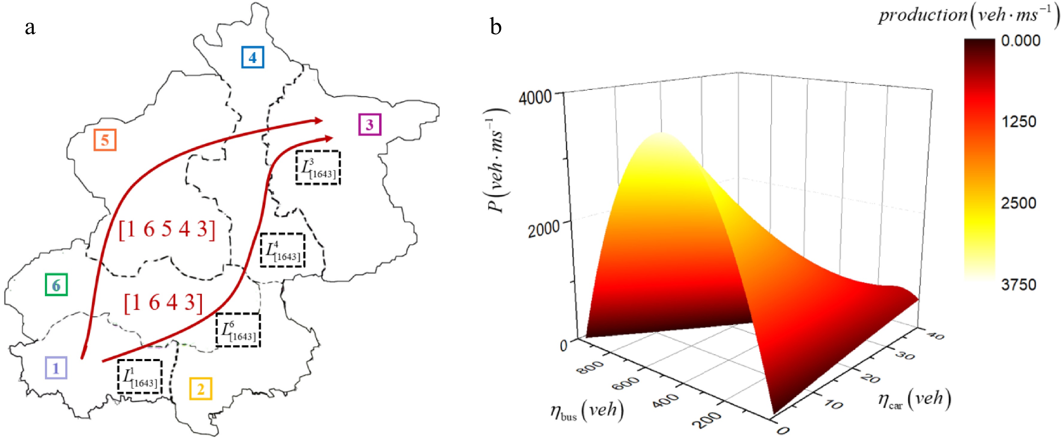
Figure 1.
A multi-reservoir network. (a) Network partitioning and characteristics. (b) 3D-MFD surface which the formula refers to Paipuri & Leclercq[27].
Assumption 2: Buses' free flow speed is lower than cars. The bus would travel at free-flow speed if the car speed is not lower than the bus speed. This assumption means the bus and the cars share the urban road space. The 3D-MFD shows the impacts of bus flow on the private cars. The bus speed would not be influenced by cars unless the car speed is lower than the bus free-flow speed.
Assumption 3: Travelers' behaviors follow a DUE rule. This assumption indicates that the travelers make decisions on modal and routing choices based on network performances.
A regional path (macroscopic path)
$p$ $r$ $p$ ${L_{{\text{p,r}}}}$ $R$ $p$ $p$ $ {L_{\text{p}}} = \sum\nolimits_{{\text{r}} \in {\text{R}}} {{L_{{\text{p,r}}}}} $ ${L_{{\text{p,r}}}}$ ${L_{\left[ {1643} \right]}}$ $L_{[1643]}^1$ $L_{[1643]}^6$ $L_{[1643]}^4$ $L_{[1643]}^6$ $T$ $K = \left\{ {k = 1,2, \ldots ,\underset{\raise0.3em\hbox{$\smash{\scriptscriptstyle-}$}}{K} } \right\}$ $\delta t$ $ \delta t\underset{\raise0.3em\hbox{$\smash{\scriptscriptstyle-}$}}{K} = T $ -
In this section, we present a macroscopic methodological framework considering two different travel modes. To simulate the traffic dynamics, the accumulation-based model is used for cars, the trip-based model is used for buses. The accumulation of buses in one reservoir determines the MFD for cars. The bus speed is determined by the accumulation of buses and cars.
For each reservoir, traffic dynamics are described by the evolution of accumulation along different paths for each mode
$m \in \left\{ {bus,car} \right\}$ $ {\eta }_{\text{p,r}}^{\text{m}}\left(t+\delta t\right)={\eta }_{\text{p,r}}^{\text{m}}\left(t\right)+\Delta {\eta }_{\text{p,r}}^{\text{m}}\left(t\right),\quad r\in \left\{1,\dots ,N\right\},\;\;\forall p\in {P}_{\text{r}}^{\text{m}},\;\; m $ (1) where
$\delta t$ $\eta _{{\text{p,r}}}^{\text{m}}\left( t \right)$ $m \in \left\{ {bus,car} \right\}$ $p$ $r$ $t$ $\Delta \eta _{{\text{p,r}}}^{\text{m}}\left( t \right)$ $p$ $r$ $t$ $P_{\text{r}}^{\text{m}}$ Accumulation-based model for cars
-
The multi-reservoir accumulation-based model is introduced by Mariotte et al.[35], which is an extension of Yildirimoglu & Geroliminis's work[34]. For cars,
$\Delta \eta _{{\text{p,r}}}^{\text{m}}\left( t \right)$ $ \Delta {\eta }_{\text{p,r}}^{\text{car}}\left(t\right)=\delta t\cdot \left({q}_{\text{p,r,in}}^{\text{car}}\left(t\right)-{q}_{\text{p,r,out}}^{\text{car}}\left(t\right)\right),\text{ }\forall r\in \left\{1,\dots ,N\right\},\;\;\forall p\in {P}_{\text{r}}^{\text{car}} $ (2) Where
$q_{{\text{p,r,in}}}^{{\text{car}}}(t)$ $q_{{\text{p,r,out}}}^{{\text{car}}}(t)$ (i) If r is the origin reservoir but not the destination, we assume the demand generated inside the reservoir without any restrictions. The effective inflow of path
$p$ $q_{{\text{p,r,in}}}^{{\text{car}}}\left( t \right) = \lambda _{\text{p}}^{{\text{w,car}}}\left( t \right){\text{ }}$ $\lambda _{\text{p}}^{{\text{w,car}}}\left( t \right)$ $w$ $q_{{\text{p,r,out}}}^{{\text{car}}}\left( t \right)$ ${p^ + }\left( r \right)$ $q_{{\text{p,r,out}}}^{{\text{car}}}\left( t \right) = \eta _{{\text{p,r}}}^{{\text{car}}}\left( t \right)L_{{\text{k,r}}}^{{\text{car}}}/\eta _{{\text{k,r}}}^{{\text{car}}}\left( t \right)L_{{\text{p,r}}}^{{\text{car}}}\min \left( {\mu _{{\text{k,r}}}^{{\text{car}}}\left( t \right),O_{{\text{k,r}}}^{{\text{car}}}\left( t \right)} \right)$ $O_{{\text{k,r}}}^{{\text{car}}}\left( t \right)$ $\mu _{{\text{k,r}}}^{{\text{car}}}\left( t \right)$ $k$ $r$ $k$ $k = \arg \mathop {\min }\limits_{p \in {P^{\text{r}}}} \mu _{{\text{p,r}}}^{{\text{car}}}\left( t \right){\text{/}}O_{{\text{p,r}}}^{{\text{car}}}\left( t \right)$ (ii) If r is the destination reservoir but not the origin, the outflow of path
$p$ $\mu _{{\text{p,r}}}^{{\text{car}}}\left( t \right) = + \infty $ $q_{{\text{p,r,in}}}^{{\text{car}}}\left( t \right) = q_{{\text{p,}}{{\text{p}}^{{-}}}\left( {\text{r}} \right){\text{,out}}}^{{\text{car}}}\left( t \right)$ ${p^ - }\left( r \right)$ (iii) If r is neither the origin reservoir nor the destination reservoir, the calculation of effective outflow and effective inflow are referred to (i) and (ii) respectively.
(iv) If r is both origin reservoir and destination reservoir, the calculation of effective inflow and effective outflow are referred to (i) and (ii) respectively.
Now we focus on the effective inflow and effective outflow of transfer flow which passes through the boundary entering the reservoir or leaving the reservoir.
As defined by Geroliminis & Daganzo[47], the trip completion rate is proportional to the total production in each reservoir, defined as
$O = P/L$ The outflow demand
$O_{{\text{p,r}}}^{{\text{car}}}\left( t \right)$ $ O_{{\text{p,r}}}^{{\text{car}}}\left( t \right) = \left\{ {\begin{array}{*{20}{l}} {\text{ }}\dfrac{{\eta _{{\text{p,r}}}^{{\text{car}}}\left( t \right)}}{{\eta _{\text{r}}^{{\text{car}}}\left( t \right)}}\dfrac{{{{\text{P}}_{\text{r}}}\left( {\eta _{\text{r}}^{{\text{car}}}\left( t \right),\eta _{\text{r}}^{{\text{bus}}}\left( t \right)} \right)}}{{L_{{\text{p,r}}}^{{\text{car}}}}}{\text{ }}\;if\\\quad \eta _{\text{r}}^{{\text{car}}}\left( t \right) \lt \eta _{\text{r}}^{{\text{crit}}}\left( {\eta _{\text{r}}^{{\text{bus}}}\left( t \right)} \right) \\ {\dfrac{{\eta _{{\text{p,r}}}^{{\text{car}}}\left( t \right)}}{{\eta _{\text{r}}^{{\text{car}}}\left( t \right)}}\dfrac{{{\text{P}}_{\text{r}}^{{\text{crit}}}\left( {\eta _{\text{r}}^{{\text{bus}}}\left( t \right)} \right)}}{{L_{{\text{p,r}}}^{{\text{car}}}}}\;\;{\text{ otherwise}}} \end{array}} \right.{\text{ }}\forall p \in P_{\text{r}}^{{\text{car}}} $ (3) where
$L_{{\text{p,r}}}^{{\text{car}}}$ $r$ $p$ $\eta _{\text{r}}^{{\text{car}}}\left( t \right)$ $\eta _{\text{r}}^{{\text{bus}}}\left( t \right)$ ${\text{P}}_{\text{r}}^{{\text{crit}}}\left( {\eta _{\text{r}}^{{\text{bus}}}\left( t \right)} \right)$ $\eta _{\text{r}}^{{\text{crit}}}\left( {\eta _{\text{r}}^{{\text{bus}}}\left( t \right)} \right)$ The restriction outflow supply
$\mu _{{\text{p,r}}}^{{\text{car}}}\left( t \right)$ $I_{{\text{p,}}{{\text{p}}^{{ + }}}\left( {\text{r}} \right)}^{{\text{car}}}\left( t \right)$ ${{\text{P}}_{{\text{S,r}}}}$ $r$ $ {{\text{P}}_{{\text{S,r}}}}\left( {\eta _{\text{r}}^{{\text{car}}}\left( t \right),\eta _{\text{r}}^{{\text{bus}}}\left( t \right)} \right) = \left\{ {\begin{array}{*{20}{lc}} {{\text{P}}_{\text{r}}^{{\text{crit}}}\left( {\eta _{\text{r}}^{{\text{bus}}}\left( t \right)} \right){\text{ }}\;\;if\;\;{\text{ }}\eta _{\text{r}}^{{\text{car}}}\left( t \right) \lt \eta _{\text{r}}^{{\text{crit}}}\left( {\eta _{\text{r}}^{{\text{bus}}}\left( t \right)} \right)} \\ {{\text{ }}{{\text{P}}_{\text{r}}}\left( {\eta _{\text{r}}^{{\text{car}}}\left( t \right),\eta _{\text{r}}^{{\text{bus}}}\left( t \right)} \right)\;\;{\text{ otherwise }}} \end{array}} \right. $ (4) For transfer flow, the available entry supply production in reservoir
$r$ ${{\text{P}}_{{\text{S,r}}}} - \displaystyle\sum\nolimits_{p \in P_{{\text{int}}}^{\text{r}}} {L_{{\text{p,r}}}^{{\text{car}}}\lambda _{\text{p}}^{{\text{w,car}}}} $ $ \displaystyle\sum\nolimits_{p \in P_{\text{r}}^{{\text{ext}}}} {\eta _{{\text{p,r}}}^{{\text{car}}}\left( t \right)} {\text{/}}\displaystyle\sum\nolimits_{p \in P_r^{ext}} {\eta _{{\text{p,r}}}^{{\text{car}}}\left( t \right)/L_{{\text{p,r}}}^{{\text{car}}}} $ ${I^{\text{r}}}$ At the same time, considering the capacity constraints of the reservoir and the nodes at the boundary, we use the sequence of macroscopic nodes corresponding to the reservoir successions of path
$p$ $N_{\text{r}}^{{\text{bd}}}$ $n$ $n$ $P_{{\text{r,n}}}^{{\text{car}}}$ $\begin{array}{c} {\left\{ {I_{\text{p}}^{{\text{r*}}}} \right\}_{p \in P_{{\text{r,n}}}^{{\text{car}}}}} = {\text{Merge}}\left( {{{\left\{ {\lambda _{{\text{p,r}}}^{{\text{car}}}} \right\}}_{p \in P_{{\text{r,n}}}^{{\text{car}}}}},{{\left\{ {\dfrac{{\alpha _{\text{p}}^{\text{r}}}}{{\displaystyle\sum\nolimits_{k \in P_{{\text{r,n}}}^{{\text{car}}}} {\alpha _{\text{k}}^{\text{r}}} }}} \right\}}_{p \in P_{{\text{r,n}}}^{{\text{car}}}}},{D_{\text{n}}}} \right),\\\;\;{\text{ }}\forall r,\;\;\forall n \in N_{\text{r}}^{{\text{bd}}}\end{array} $ (5) where
${\text{Merge}}\left( \cdot \right)$ ${D_{\text{n}}}$ $n$ $n$ $\lambda _{{\text{p,r}}}^{{\text{car}}}$ $p$ $r$ $O_{{\text{p,}}{{\text{p}}^{{- }}}\left( {\text{r}} \right)}^{{\text{car}}}$ $\alpha _{\text{p}}^{\text{r}}$ $\lambda _{\text{p}}^{\text{r}}/\sum\nolimits_{p \in P_{{\text{r,m}}}^{{\text{car}}}} {\lambda _{\text{k}}^{\text{r}}} $ $ {\left\{ {I_{\text{p}}^{\text{r}}} \right\}_{p \in P_{{\text{r,bd}}}^{{\text{car}}}}} = {\text{Merge}}\left( {{{\left\{ {I_{\text{p}}^{{\text{r*}}}} \right\}}_{p \in P_{{\text{r,bd}}}^{{\text{car}}}}},{{\left\{ {\alpha _{\text{p}}^{\text{r}}} \right\}}_{p \in P_{{\text{r,bd}}}^{{\text{car}}}}},{I^{\text{r}}}} \right),{\text{ }}\forall r $ (6) where
$P_{{\text{r,bd}}}^{{\text{car}}}$ $r$ $I_{{\text{p,r}}}^{{\text{car}}}\left( t \right)$ Then the evolution of car accumulation is calculated by Eq. (1). At the same time, the cumulative count curves of each path in reservoir
$r$ $U_{{\text{p,in}}}^{{\text{car,o}}}\left( t \right)$ $V_{{\text{p,out}}}^{{\text{car}}{\text{.d}}}\left( t \right)$ $p$ $t$ ${\tau _{{\text{p,car}}}}\left( t \right)$ $t$ $p$ $ \begin{gathered} U_{{\text{p,r,in}}}^{{\text{car}}}\left( t \right) = \int_0^t {q_{{\text{p,r,in}}}^{{\text{car}}}\left( t \right)} dt + \eta _{{\text{p,r}}}^{{\text{car}}}\left( 0 \right)\quad\forall r \in \left\{ {1, \ldots ,N} \right\},p \in P_{\text{r}}^{{\text{car}}} \\ V_{{\text{p,r,out}}}^{{\text{car}}}\left( t \right) = \int_0^t {q_{{\text{p,r,out}}}^{{\text{car}}}\left( t \right)} dt \\ \end{gathered} $ (7) The relationship between travel time and cumulative flow is:
$ U_{{\text{p,r,in}}}^{{\text{car}}}\left( {t - {\tau _{{\text{p,car}}}}\left( t \right)} \right) = V_{{\text{p,r,out}}}^{{\text{car}}}\left( t \right) $ (8) If
$U_{\rm p,in}^{\rm car,o}\left( t \right)$ $V_{{\text{p,out}}}^{{\text{car,d}}}\left( t \right)$ $t$ $ {\tau _{{\text{p,car}}}}\left( t \right) = t - U{_{{\text{p,in}}}^{{\rm{car,o{\text -}1}}}}\left( {V_{{\text{p,out}}}^{{\text{car,d}}}\left( t \right)} \right) $ (9) where
${U_{{\rm{p,in}}}^{{\rm{car,o{\text -}1}}}}\left( \cdot \right)$ $U_{{\rm{p,in}}}^{{\rm{car,o}}}\left( \cdot \right)$ Here, the travel time of each path
$p$ ${\tau _{{\text{p,car}}}}\left( t \right)$ Trip-based model for buses
-
All buses are traveling at the same speed
$v_{\text{r}}^{{\text{bus}}}\left( {\eta _{\text{r}}^{{\text{car}}}\left( t \right),\eta _{\text{r}}^{{\text{bus}}}\left( t \right)} \right)$ $r$ $t$ $p$ $r$ $ L_{{\text{p,r}}}^{{\text{bus}}} = \int_{t - T\left( t \right)}^t {v_{\text{r}}^{{\text{bus}}}\left( {\eta _{\text{r}}^{{\text{car}}}\left( t \right),\eta _{\text{r}}^{{\text{bus}}}\left( t \right)} \right)dt} $ (10) where
$L_{{\text{p,r}}}^{{\text{bus}}}$ $r$ $p$ $t - T\left( t \right)$ $t$ $v_{\text{r}}^{{\text{bus}}}\left( {\eta _{\text{r}}^{{\text{car}}}\left( t \right),\eta _{\text{r}}^{{\text{bus}}}\left( t \right)} \right)$ $t$ $v_{\text{r}}^{{\text{bus}}}$ $ v_{\text{r}}^{{\text{bus}}}\left( {\eta _{\text{r}}^{{\text{car}}},\eta _{\text{r}}^{{\text{bus}}}} \right) = {\beta _{{\text{b,0}}}} + {\beta _{{\text{c,b}}}}\eta _{\text{r}}^{{\text{car}}}\left( t \right) + {\beta _{{\text{b,b}}}}\eta _{\text{r}}^{{\text{bus}}}\left( t \right) $ (11) Constants
${\beta _{{\text{c,b}}}}$ ${\beta _{{\text{b,b}}}}$ We track the bus trip distance until the total trip length
$L_{\text{p}}^{{\text{bus}}} = \displaystyle\sum\limits_{r \in R} {L_{{\text{p,r}}}^{{\text{bus}}}} $ ${\tau _{{\text{p,bus,travel}}}}$ $\Delta \eta _{{\text{p,r}}}^{\text{m}}\left( t \right)$ $ \Delta {\eta }_{\text{p,r}}^{\text{bus}}\left(t\right)={\eta }_{\text{p,r,in}}^{\text{bus}}\left(t\right)-{\eta }_{\text{p,r,out}}^{\text{bus}}\left(t\right),\quad\forall r\in \left\{1,\dots ,N\right\},\;\;\forall p\in {P}_{\text{r}}^{\text{bus}} $ (12) Where
$\eta _{{\text{p,r,in}}}^{{\text{bus}}}\left( t \right)$ $\eta _{{\text{p,r,out}}}^{{\text{bus}}}\left( t \right)$ $r$ $p$ $t$ ${p^+}\left( r \right)$ $\eta _{{\text{p,}}{{\text{p}}^ + }\left( {\text{r}} \right){\text{,in}}}^{{\text{bus}}}\left( t \right) = \eta _{{\text{p,r,in}}}^{{\text{bus}}}\left( {t - T\left( t \right)} \right)$ $r$ $\eta _{{\text{p,r,out}}}^{{\text{bus}}}\left( t \right) = \eta _{{\text{p,}}{{\text{p}}^ + }\left( {\text{r}} \right){\text{,in}}}^{{\text{bus}}}\left( {t - T\left( t \right)} \right)$ Table 1. Trip-based solver algorithm.
Input: Reservoir initial bus accumulation $\eta _{{\text{p,r}}}^{{\text{bus}}}\left( {{t_0}} \right)$ of each path, car accumulation $\eta _{{\text{p,r}}}^{{\text{car}}}\left( {{t_0}} \right)$ of each path, initial trip distance $L_{{\text{p,r,t}}}^{{\text{bus}}}\left( {{t_{\text{0}}}} \right){\text{ = 0}}$, the subscript $t$ represents the bus departing at time $t$, traffic demand profile $\lambda _{\text{p}}^{{\text{w,bus}}}\left( t \right)$, simulation duration $T$ and time step $\delta t$. 1: for $t = {t_0}$ to ${t_0} + T$ by $\delta t$ do 2: According to the bus and car accumulation which is calculated by Eq. (1), combined with reservoir 3D-MFD, the bus speed $v_{\text{r}}^{{\text{bus}}}\left( t \right)$ is determined by Eq. (11) 3: for $r = 1$ to $N$ do 4: Inflow: if $r = o$ then $\eta _{{\text{p,r,in}}}^{{\text{bus}}}\left( t \right) = \lambda _{\text{p}}^{{\text{w,bus}}}\left( t \right) \cdot \delta t$ else $\eta _{{\text{p,r,in}}}^{{\text{bus}}}\left( t \right) = \eta _{{\text{p,}}{{\text{p}}^{\text{ - }}}\left( {\text{r}} \right){\text{,out}}}^{{\text{bus}}}\left( t \right)$ 5: Outflow: track the trip distance $L_{{\text{p,r,t}}}^{{\text{bus}}}\left( {t{\text{ + }}\delta t} \right) = L_{{\text{p,r,t}}}^{{\text{bus}}}\left( t \right) + v_{\text{r}}^{{\text{bus}}}\left( t \right) \cdot \delta t$ 6: if $L_{{\text{p,r,t}}}^{{\text{bus}}}\left( {t{\text{ + }}\delta t} \right) > L_{{\text{p,r}}}^{{\text{bus}}}$ 7: if $r = d$ then $ {\tau _{{\text{p,bus,travel}}}}\left( t \right) = {\tau _{{\text{p,bus,travel}}}}\left( t \right) + {t_{\text{s}}} $, $\eta _{{\text{p,r,out}}}^{{\text{bus}}}\left( t \right) = \eta _{{\text{p,r,in}}}^{{\text{bus}}}\left( {t{\text{ - }}{\tau _{{\text{p,bus,travel}}}}\left( t \right)} \right)$
where ${t_{\text{s}}}$ is the traveling time in reservoir $r$.8: else ${\tau _{{\text{p,bus,travel}}}}\left( t \right) = {\tau _{{\text{p,bus,travel}}}}\left( t \right) + \delta t$, $\eta _{{\text{p,r,out}}}^{{\text{bus}}}\left( t \right) = \eta _{{\text{p,r,in}}}^{{\text{bus}}}\left( {t{\text{ - }}{\tau _{{\text{p,bus,travel}}}}\left( t \right)} \right)$ 9: else ${\tau _{{\text{p,bus,travel}}}}\left( t \right) = {\tau _{{\text{p,bus,travel}}}}\left( t \right) + \delta t$, $\eta _{{\text{p,r,out}}}^{{\text{bus}}}\left( t \right) = 0$ 10: Bus accumulation update: $\eta _{{\text{p,r}}}^{{\text{bus}}}\left( {t + \delta t} \right) = \eta _{{\text{p,r}}}^{{\text{bus}}}\left( t \right) + \eta _{{\text{p,r,in}}}^{{\text{bus}}}\left( t \right) - \eta _{{\text{p,r,out}}}^{{\text{bus}}}\left( t \right)$ 11: end for 12: end for Output: reservoir bus accumulation $\eta _{{\text{p,r}}}^{{\text{bus}}}\left( t \right)$, the experienced travel time ${\tau _{{\text{p,bus,travel}}}}\left( t \right)$ In this paper, the travel time along path
$p$ $p \in P_{{\text{bus}}}^{\text{w}}$ ${\tau _{{\text{p,bus,travel}}}}\left( t \right)$ $\tau _{{\rm{p,bus,\omega ait}}}^{\text{w}}$ -
First we establish a bi-level optimization framework. The upper-level problem minimizes the total time spent of all road users and bus operation cost. The lower-level problem is a region-based dynamic traffic assignment model.
Bi-level optimization framework
-
The bus optimization problem in a large-scale transportation network is formulated in a bi-level programming framework. The upper-level determines the optimal frequencies, while the lower level determines traffic behaviour decisions, which is formulated as a multi-modal DUE model with a 3D-MFD based network loading model.
Upper-level problem
-
We consider the total time spent of all road users and the bus operation cost in the upper-level model. The upper-level model is expressed as follows:
$ \min Z\left( {\mathbf{F}} \right) = \alpha \beta {T_{{\text{system}}}} + \left( {{\text{1 - }}\alpha } \right){C_{{\text{operation}}}} $ (13) $ {\text{s}}{\text{.t}}{\text{. }}\sum\limits_{w \in W} {\sum\limits_{p \in P_{{\text{bus}}}^{\text{w}}} {N_{\text{p}}^{\text{w}}\left( {{\text{F}}_{\text{p}}^{\text{w}}} \right) \cdot G_{\text{p}}^{\text{w}}} \leqslant B} {\text{ }} $ (14) $ {\text{ F}}_{\text{p}}^{\text{w}} \in {F_{\text{p}}},{\text{ }}{F_{\text{p}}} = \left\{ {{\text{F}}_{\text{p}}^{\text{1}},{\text{F}}_{\text{p}}^{\text{2}}, \ldots ,{\text{F}}_{\text{p}}^{\text{n}}} \right\} $ (15) where
$Z\left( {\mathbf{F}} \right)$ ${\mathbf{F}}$ ${\mathbf{F}} = \left\{ {{{\mathbf{F}}^{\text{w}}},w \in W} \right\}$ ${T_{{\text{system}}}}$ ${C_{{\text{operation}}}}$ $\left( {{\text{person}} \cdot \min } \right)$ $\left( {\$} \right)$ $\alpha $ $1 - \alpha $ $\beta $ $\beta = 1.0{\$} /{\text{person}} \cdot \min $ (1) Total time spent of passengers
${T_{{\text{system}}}}$ The total time spent is the product of the passenger flow and the corresponding path travel time of all paths. It is used to evaluate the bus frequency improvement on the network performance.
$ {T_{{\text{system}}}} = \sum\limits_{t \in T} {\sum\limits_{w \in W} {\sum\limits_{p \in {P^{\text{w}}}} {f_{\text{p}}^{\text{w}}\left( {{\mathbf{F}},t} \right) \cdot \tau _{\text{p}}^{\text{w}}\left( {f_{\text{p}}^{\text{w}}\left( {{\mathbf{F}},t} \right),t} \right)} } } $ (16) The passenger flow
$f_{\text{p}}^{\text{w}}\left( {{\mathbf{F}},t} \right)$ $\tau _{\text{p}}^{\text{w}}\left( {f_{\text{p}}^{\text{w}}\left( {{\mathbf{F}},t} \right),t} \right)$ (2) Operating cost of buses
${C_{{\text{operation}}}}$ Energy consumption, vehicle depreciation, personnel wages and so on should be considered in the operation cost. This paper assumes that the average single trip operation cost
$G_{\text{p}}^{\text{w}}$ $ {C_{{\text{operation}}}} = \sum\limits_{w \in W} {\sum\limits_{p \in P_{{\text{bus}}}^{\text{w}}} {N_{\text{p}}^{\text{w}}\left( {{\text{F}}_{\text{p}}^{\text{w}}} \right) \cdot G_{\text{p}}^{\text{w}}} } $ (17) where
$N_{\text{p}}^{\text{w}}$ $p$ $p \in P_{{\text{bus}}}^{\text{w}}$ (3) Constraint condition
Due to the limited number of buses by bus operations, the constraint condition is Eq. (15), and the operating cost cannot exceed the budget
$B$ $\left\{ {{\text{F}}_{\text{p}}^{\text{1}},{\text{F}}_{\text{p}}^{\text{2}}, \ldots ,{\text{F}}_{\text{p}}^{\text{n}}} \right\}$ ${\text{f}}_{\text{p}}^{\text{w}}$ $p \in P_{{\text{bus}}}^{\text{w}}$ ${\text{F}}_{\text{p}}^{\text{w}} \in {F_{\text{p}}},{F_{\text{p}}} = \left\{ {{\text{F}}_{\text{p}}^{\text{1}},{\text{F}}_{\text{p}}^{\text{2}}, \ldots ,{\text{F}}_{\text{p}}^{\text{n}}} \right\}$ Lower-level problem
-
In this paper, the bus lines and car routes are considered as paths. Travelers choose ones' travel mode and path following the DUE rule. The travel time of bus passengers include in-vehicle time and the waiting time at bus stops. In this model, the OD demand is time-dependent. Considering the time discretization, the DUE condition of the whole network is established as follows:
$ \begin{gathered} \tau _{{\text{p,m}}}^{\text{w}}\left( k \right) - \mu _{\text{m}}^{\text{w}}\left( k \right) = 0{\text{ if }}\forall p \in P_{\text{m}}^{\text{w}},k \in K,{\text{ }}f_{{\text{p,m}}}^{\text{w}}\left( k \right) \gt 0 \\ \tau _{{\text{p,m}}}^{\text{w}}\left( k \right) - \mu _{\text{m}}^{\text{w}}\left( k \right) \geqslant 0{\text{ if }}\forall p \in P_{\text{m}}^{\text{w}},k \in K,{\text{ }}f_{{\text{p,m}}}^{\text{w}}\left( k \right) = 0 \\ \end{gathered} $ (18) where
$ \mu _{\text{m}}^{\text{w}}\left( k \right) $ $ m \in \left\{ {bus,car} \right\} $ $w$ $k$ $ f_{{\text{p,m}}}^{\text{w}}\left( k \right) $ $ p $ $ m $ $w$ $k$ $ m $ $w$ $ {\lambda ^{\text{w}}}\left( k \right) = \displaystyle\sum\limits_{m \in \left\{ {bus,car} \right\}} {\displaystyle\sum\limits_{p \in P_{\text{m}}^{\text{w}}} {f_{{\text{p,m}}}^{\text{w}}\left( k \right)} } $ $w$ ${\lambda ^{\text{w}}}\left( k \right)$ $\tau _{{\text{p,m}}}^{\text{w}}\left( k \right)$ $f_{{\text{p,m}}}^{\text{w}}\left( k \right)$ The DUE condition can be formulated as a variational inequality model. The variables are the path flows, which can be described as Eq. (17). Let
${\mathbf{f}}$ $ \sum\limits_{k \in K} {\sum\limits_{w \in W} {\sum\limits_{p \in {P_w}} {\tau {{_{\text{p}}^{\text{w}}}^ * }\left( k \right)\left[ {f_{\text{p}}^{\text{w}}\left( k \right) - f{{_{\text{p}}^{\text{w}}}^ * }\left( k \right)} \right] \geqslant 0} ,\;{\text{ }}\forall {\mathbf{f}} \in \Omega } } $ (19) Among which
$\Omega = \left\{ {{\mathbf{f}} \geqslant 0\left| {\displaystyle\sum\nolimits_{p \in {P_{\text{w}}}} {f_{\text{p}}^{\text{w}}\left( k \right) = {\lambda ^{\text{w}}}\left( k \right)} ,{\text{ }}\forall w \in W, \; k \in K} \right.} \right\}$ $\tau _{\text{p}}^{\text{w}}$ $\tau _{{\text{p,car}}}^{\text{w}}$ $\tau _{{\text{p,bus}}}^{\text{w}}$ $w$ $p$ $\tau _{{\text{p,car}}}^{\text{w}}$ $\begin{array}{c} \tau _{{\text{p,bus}}}^{\text{w}}\left( {f_{{\text{p,bus}}}^{\text{w}}\left( {{\mathbf{F}},k} \right),k} \right) = \tau _{{\text{p,bus,travel}}}^{\text{w}}\left( {{\mathbf{F}},k} \right) + \tau _{{\rm{p,bus,\omega ait}}}^{\text{w}}\left( {{\mathbf{F}},k} \right),\\\forall p \in P_{{\text{bus}}}^{\text{w}},\;\;k \in K,\;\;w \in W \end{array}$ (20) where
$\tau _{{\text{p,bus,travel}}}^{\text{w}}\left( {{\mathbf{F}},k} \right)$ $p \in P_{{\text{bus}}}^{\text{w}}$ ${\mathbf{F}}$ $\tau _{{\rm{p,bus,\omega ait}}}^{\text{w}}\left( {{\mathbf{F}},k} \right)$ $p$ $ \tau _{{\rm{p,bus,\omega ait}}}^{\text{w}}\left( {{\mathbf{F}},k} \right) = \frac{{\displaystyle\sum\limits_{a = 1}^{f_{{\text{p,bus}}}^{\text{w}}\left( t \right)} {{\tau _{\text{p}}}\left( a \right)} }}{{f_{{\text{p,bus}}}^{\text{w}}\left( k \right)}},\;\;\forall p \in P_{{\text{bus}}}^{\text{w}},\;\;k \in K,\;\;w \in W $ (21) where
${\tau _{\text{p}}}\left( a \right)$ $a{\text{ th}}$ $p \in P_{{\text{bus}}}^{\text{w}}$ -
In this section, we use a double projection algorithm approach to solve the lower-level problem which is formulated as a variational inequality. The surrogate model algorithm is designed to solve the proposed bus frequency optimization problem.
Double projection algorithm used to solve the VI model
-
The double projection algorithm is used to solve the dynamic traffic assignment problem in our proposed model, see Algorithm 2. The double projection algorithm is a modified method to solve large-scale VI problems. This method avoids the drawback of slow convergence due to consistently small iteration step size. The reinitialization of the step size
${\rho ^{\text{γ }}}$ $\text{pro}{\text{j}}_{\Omega}$ $\Omega $ ${{\mathbf{f}}^{\text{γ }}}(k)$ ${\mathbf{\tau }}({{\mathbf{f}}^{\text{γ }}}(k))$ $\gamma $ $k$ Table 2. Double projection algorithm.
Input: projection step $\bar \rho $, accuracy $\varepsilon > 0$, select parameters $\beta $, $ \xi \in \left(\text{0},\text{1}\right) $, path set ${P^{\text{w}}}$ 1: Initial path demand ${{\mathbf{f}}^0}\left( k \right) = {\lambda ^{\text{w}}}\left( k \right)/\varsigma $, $\varsigma $ is the sum of path between OD pair $w$, the dynamic travel
time ${\mathbf{\tau }}$ of all path is obtained in section "Lower-level problem". Set ${\rho ^0} = \bar \rho $, iteration $\gamma = 0$.2: while $G({{\mathbf{f}}^{\text{γ }}}) > \varepsilon $ 3: Compute ${{\mathbf{\bar f}}^{\text{γ }}}(k) = {\text{pro}}{{\text{j}}_\Omega }({{\mathbf{f}}^{\text{γ }}}(k) - {\rho ^{\text{γ }}}{\mathbf{\tau }}({{\mathbf{f}}^{\text{γ }}}(k)))$ 4: while ${\rho ^{\text{γ }}} > \beta \frac{{\left\| {{{\mathbf{f}}^{\text{γ }}}(k) - {{{\mathbf{\bar f}}}^{\text{γ }}}(k)} \right\|}}{{\left\| {{\mathbf{\tau }}({{\mathbf{f}}^{\text{γ }}}(k)) - {\mathbf{\tau }}({{{\mathbf{\bar f}}}^{\text{γ }}}(k))} \right\|}}$ do 5: ${\rho ^{\text{γ }}} = \min \left\{ {\xi {\rho ^{\text{γ }}},\beta \frac{{\left\| {{{\mathbf{f}}^{\text{γ }}}(k) - {{{\mathbf{\bar f}}}^{\text{γ }}}(k)} \right\|}}{{\left\| {{\mathbf{\tau }}({{\mathbf{f}}^{\text{γ }}}(k)) - {\mathbf{\tau }}({{{\mathbf{\bar f}}}^{\text{γ }}}(k))} \right\|}}} \right\}$ 6: Compute ${{\mathbf{\bar f}}^{\text{γ }}}(k) = {\text{pro}}{{\text{j}}_\Omega }({{\mathbf{f}}^{\text{γ }}}(k) - {\rho ^{\text{γ }}}{\mathbf{\tau }}({{\mathbf{f}}^{\text{γ }}}(k)))$ 7: end while 8: Compute ${{\mathbf{f}}^{{\text{γ + 1}}}}(k) = {\text{pro}}{{\text{j}}_\Omega }({{\mathbf{f}}^{\text{γ }}}(k) - {\rho ^{\text{γ }}}{\mathbf{\tau }}({{\mathbf{\bar f}}^{\text{γ }}}(k)))$ 9: Update travel time vector ${\mathbf{\tau }}({{\mathbf{f}}^{\gamma + 1}}(k))$ by the dynamic network loading models in previous section. Set $\gamma = \gamma + 1$ 10: end while Output: flow vector ${{\mathbf{f}}^{\text{γ }}}(k)$ To evaluate the accuracy of solutions in each iteration in the double projection algorithm, a gap function is required, see Eq. (23).
$ G\left( {\mathbf{f}} \right) = 1 - \frac{{\displaystyle\sum\limits_{k \in K} {\displaystyle\sum\limits_{w \in W} {{\lambda ^{\text{w}}}\left( k \right){u^{\text{w}}}\left( k \right)} } }}{{\displaystyle\sum\limits_{k \in K} {\sum\limits_{w \in W} {\displaystyle\sum\limits_{p \in {P^{\text{w}}}} {f_{\text{p}}^{\text{w}}\left( k \right)\tau _{\text{p}}^{\text{w}}\left( k \right)} } } }} $ (22) Where
$ {u^{\text{w}}}(k) $ $w$ $k$ $ G({\mathbf{f}}) \leqslant \varepsilon $ $\varepsilon $ Surrogate model-based algorithm use to solve the bi-level programming problem
-
Consider M bus lines in the network and N alternative bus frequencies. We can generate
${N^{\text{M}}}$ The solution of bus optimization problem is expressed as vector
${\mathbf{y}}$ ${\mathbf{Z}}$ $w_n^s$ ${\gamma _{\max }}$ Table 3. Surrogate model-based algorithm.
Input: the maximum iterations ${\gamma _{\max }}$, the maximum consecutive successes $ C_{{\text{success}}}^{{\text{max}}} $, the maximum consecutive failures $ C_{{\text{fail}}}^{{\text{max}}} $, the initial disturbance probability $ p_{{\text{slct}}}^{{\text{init}}} $. 1: Initialization 1.1 initial evaluation points set. ${I_0} = \left\{ {{{\mathbf{y}}_1},{{\mathbf{y}}_2}, \ldots ,{{\mathbf{y}}_{{{\text{n}}_{\text{0}}}}}} \right\}$, the number of evaluation points is ${n_0}$, the real objective function value vector ${\mathbf{Z}} = \left[ {Z\left( {{{\mathbf{y}}_{\text{i}}}} \right),{{\mathbf{y}}_{\text{i}}} \in {I_0}} \right]$ corresponding to each evaluation point ${{\mathbf{y}}_{\text{i}}} = \left\{ {{{\left\{ {{f_1},{f_2}, \ldots ,{f_{{{\text{n}}_{\text{0}}}}}} \right\}}^{\text{i}}}} \right\}$ (evaluation point is the bus frequency planning of each line) is calculated, and the best feasible solution with the minimum objective value $Z\left( {{{\mathbf{y}}_{\text{i}}}} \right)$ as the current optimal solution ${{\mathbf{y}}_{{\text{best}}}}$, set the iterate number $\gamma = 0$. 1.2 initialization parameters. Initialize the counters of consecutive successes ${C_{{\text{sucess}}}} = 0$, the counters of consecutive failures ${C_{{\text{fail}}}} = 0$, the maximum number of consecutive updating success and failure of the optimal solution are $C_{{\text{success}}}^{\max }$ and $C_{{\text{fail}}}^{{\text{max}}}$, set the disturbance probability $p_{{\text{slct}}}^{\text{0}} = p_{{\text{slct}}}^{{\text{init}}}$. 2: Repeat 3: Update surrogate model.
Use the evaluation point set ${I_{\text{n}}}$ and Eq. (14) to calculate the corresponding objective function value ${\prod _{\text{n}}} = \left\{ {\left( {{{\mathbf{y}}_{\text{i}}},Z\left( {{{\mathbf{y}}_{\text{i}}}} \right)} \right),{{\mathbf{y}}_{\text{i}}} \in {I_{\text{n}}}} \right\}$, and update the surrogate model ${S_{\text{n}}}\left( {\mathbf{y}} \right)$ refer to Liu[50].4: Candidate points set generation.
Based on the perturbation probability $ {p_{{\text{slc}}t}} $, the candidate points set ${E_{\text{n}}}$ is generated by perturbing the value of any variable in the current optimal solution ${{\mathbf{y}}_{{\text{best}}}}$. When generating candidate points, ensure that each candidate point meets the investment constraint Eq. (15).5: Select the evaluation point.
Each candidate point is scored. Set ${{\mathbf{y}}_{{\text{n+1}}}}$ as the best candidate and calculate $Z({{\mathbf{y}}_{{\text{n+1}}}})$.7: Update the optimal solution.
If $Z({{\mathbf{y}}_{{\text{n+1}}}}) < Z({{\mathbf{y}}_{{\text{best}}}})$, then update the optimal solution ${{\mathbf{y}}_{{\text{best}}}} = {{\mathbf{y}}_{{\text{n+1}}}}$ and $Z({{\mathbf{y}}_{{\text{best}}}}){\text{ = }}Z({{\mathbf{y}}_{{\text{n+1}}}})$, continuous success iteration ${C_{{\text{success}}}} = {C_{{\text{success}}}} + 1$ and continuous failure iteration ${C_{{\text{fail}}}} = 0$; otherwise, let ${C_{{\text{fail}}}} = {C_{{\text{fail}}}} + 1$ and ${C_{{\text{success}}}} = 0$.8: Adjust disturbance probability.
If $ {C_{{\text{success}}}} > C_{{\text{success}}}^{{\text{max}}} $, then $ p_{{\text{slct}}}^{{\text{n+1}}} = \min \{ 2p_{{\text{slct}}}^{\text{n}},p_{{\text{slct}}}^{{\text{max}}}\} $, $ {C_{{\text{success}}}} = 0 $.
If $ {C_{{\text{fail}}}} > C_{{\text{fail}}}^{{\text{max}}} $, set $ p_{{\text{slct}}}^{{\text{n+1}}} = \max \{ p_{{\text{slct}}}^{\text{n}}/2,p_{{\text{slct}}}^{{\text{min}}}\} $ and $ {C_{{\text{fail}}}} = 0 $. Set $\gamma = \gamma + 1$.9: Update the evaluation points set.
${I_{{\text{n+1}}}} = {I_{\text{n}}} \cup \{ {{\mathbf{y}}_{{\text{n+1}}}}\} $10: Until $\gamma \geqslant {\gamma _{\max }}$ Output: ${{\mathbf{y}}_{{\text{best}}}}$ -
In this section, we conduct numerical case studies to test the performance of the proposed large-scale bus frequency optimization framework. The studied network and simulation scenarios are described in the Network structure section. The simulation results are given in the Results section. We firstly display the convergence of double projection algorithm, the result of dynamic traffic assignment, and the network traffic dynamics. Then we display the convergence process of surrogate model-based algorithm. Furthermore, we compare the optimal results in four scenarios and show the effect of our proposed model considering 3D-MFD and dynamic user equilibrium. All experiments are run on a computer with an Intel(R) Core (TM) i7 3.60 GHz and 16.0 GB RAM.
Network structure
-
The case study network consists of six reservoirs, including two regional OD pairs (1-6, 2-5) and eight paths (four car routes and four bus lines), as shown in Fig. 2. Each reservoir has a well-defined 3D-MFD. The 3D-MFD used in this paper as shown in Fig. 1b. The macroscopic paths sequence are as follows: four car routes
$\left[ {{R_1}{\text{ }}{R_2}{\text{ }}{R_3}{\text{ }}{R_6}} \right]$ $\left[ {{R_1}{\text{ }}{R_4}{\text{ }}{R_5}{\text{ }}{R_6}} \right]$ $\left[ {{R_2}{\text{ }}{R_5}} \right]$ $\left[ {{R_2}{\text{ }}{R_3}{\text{ }}{R_6}{\text{ }}{R_5}} \right]$ $\left[ {{R_1}{\text{ }}{R_2}{\text{ }}{R_3}{\text{ }}{R_6}} \right]$ $\left[ {{R_1}{\text{ }}{R_4}{\text{ }}{R_5}{\text{ }}{R_6}} \right]$ $\left[ {{R_2}{\text{ }}{R_1}{\text{ }}{R_4}{\text{ }}{R_5}} \right]$ $\left[ {{R_2}{\text{ }}{R_3}{\text{ }}{R_6}{\text{ }}{R_5}} \right]$ $\delta t$ 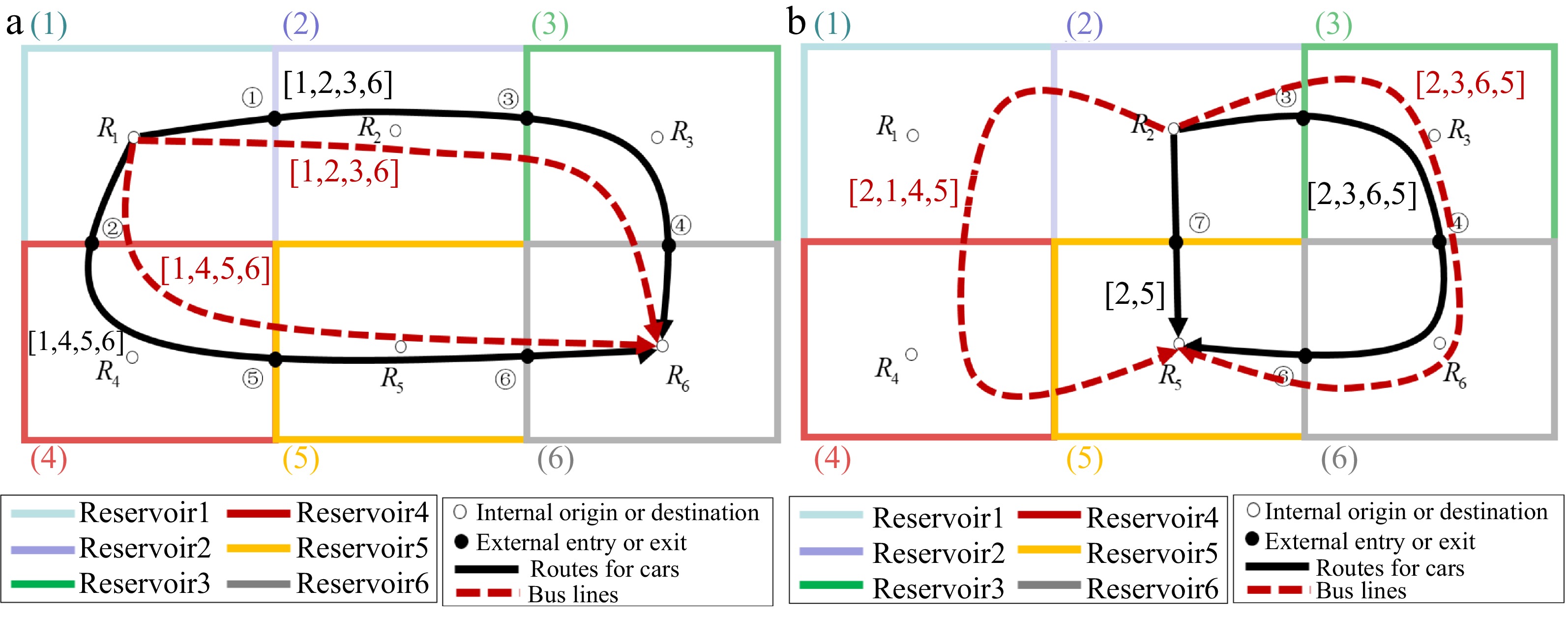
Figure 2.
Reservoir system configuration. (a) The regional OD pair (1−6). (b) The regional OD pair (2−5).
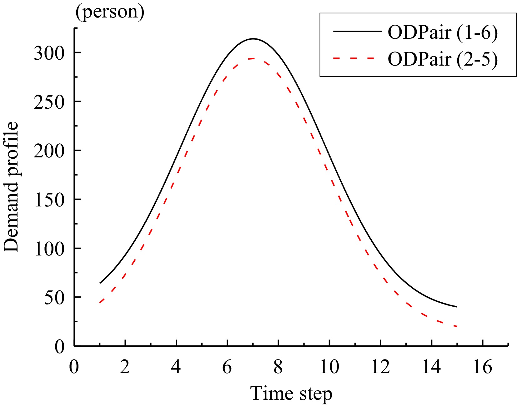
Figure 3.
OD demand profile.
The trip lengths in each reservoir by different paths are referred to in Mariotte & Leclercq[42]. For the method of estimating the trip length, we refer to Batista et al.[46] and Mariotte et al.[35]. The reservoir characteristics
$L_{\text{p}}^{\text{m}}$ Table 1. Reservoir characteristics, where $L_{\text{1}}^{{\text{car}}}$, $L_{\text{2}}^{{\text{car}}}$, $L_3^{{\text{car}}}$, $L_{\text{4}}^{{\text{car}}}$ refer to the trip length of route 1, 2, 3, 4 and $L_{\text{1}}^{{\text{bus}}}$, $L_{\text{2}}^{{\text{bus}}}$, $L_{\text{3}}^{{\text{bus}}}$, $L_{\text{4}}^{{\text{bus}}}$ refer to the trip length of bus line 1, 2, 3, 4.
Characteristics [units] ${R_1}$ ${R_2}$ ${R_3}$ ${R_4}$ ${R_5}$ ${R_6}$ Trip length $L_{\text{1}}^{{\text{car}}}$ [m] 2500 5000 5000 − − 2500 Trip length $L_{\text{2}}^{{\text{car}}}$ [m] 2500 − − 5000 5000 2500 Trip length $L_3^{{\text{car}}}$ [m] − 2500 − − 2500 − Trip length $L_{\text{4}}^{{\text{car}}}$ [m] − 2500 5000 − 2500 5000 Bus line $L_{\text{1}}^{{\text{bus}}}$ [m] 2500 5000 5000 − − 2500 Bus line $L_{\text{2}}^{{\text{bus}}}$ [m] 2500 − − 5000 5000 3500 Bus line $L_{\text{3}}^{{\text{bus}}}$ [m] 5000 2500 − 5000 2500 − Bus line $L_{\text{4}}^{{\text{bus}}}$ [m] − 2500 5000 − 2500 5000 In the numerical study, the trip operation cost
$G_{\text{p}}^{\text{w}} = 300{\$} /{\rm {veh}}$ $p$ $B = 100000{\$} $ $\beta = 1.0{\$} /{\text{veh}} \cdot \min $ ${p_{{\text{slct}}}} = 0.8$ $w_{\text{n}}^{\text{S}} = 0.6$ ${\gamma _{\max }} = 100$ In particular, we analyze the simulation results when
$\alpha = 0.5$ We compare the optimal solution and results in four scenarios:
Scenario 1: Considering 2D-MFD based model and non-equilibrium condition.
Scenario 2: Considering 2D-MFD based model and equilibrium condition.
Scenario 3: Considering 3D-MFD based model and non-equilibrium condition.
Scenario 4: Considering 3D-MFD based model and equilibrium condition.
We optimize the 2D-MFD for each reservoir based on the results obtained by fitting (parabolic fitting) which match the production-MFD well[35]. The data points are based on the relationship between the production and the accumulation of vehicles in each reservoir obtained by 3D-MFD simulation. The correlation coefficient is expressed as
${R^2}$ Results
Properties of our proposed model
Convergence process of double projection algorithm
-
The convergence process of the double projection algorithm to solve the DTA problem is shown in Fig. 4. A stationary Gap value has been reached in 400 iterations.
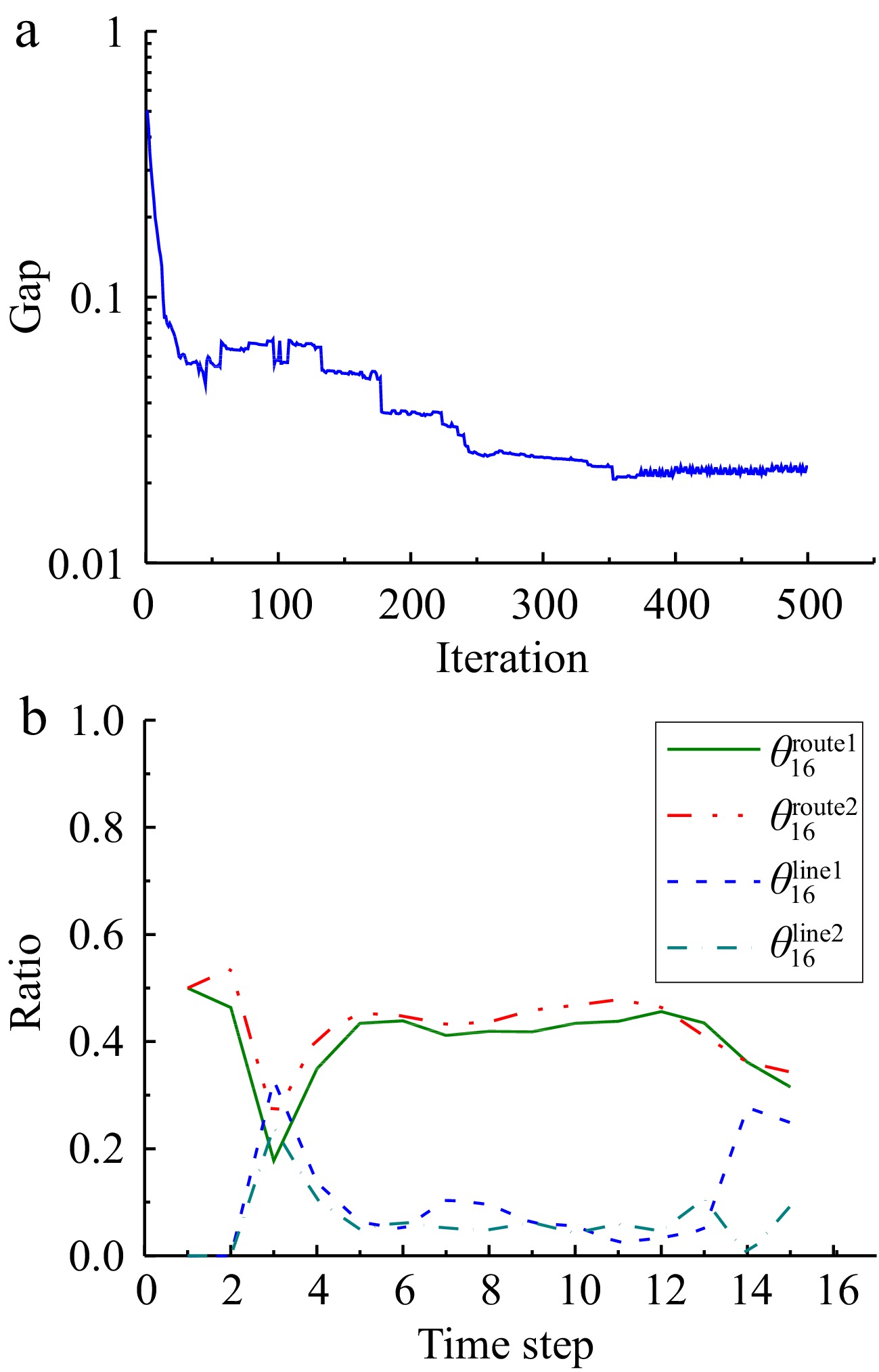
Figure 4.
Results using double projection algorithm. (a) Convergence of double projection algorithm. (b) Route choice parameters for an OD pair.
Using the double projection algorithm, the mode and route choices of all users at each time can be obtained in Fig. 4b, the proportion of demand between origin 1 and destination 6 that chooses different routes are given. The proportion of demand between OD that choose the route
$p$ $\theta _{{\text{od}}}^{\text{p}}$ $\theta _{{\text{16}}}^{{\text{route1}}}$ $\theta _{{\text{16}}}^{{\text{line1}}}$ Traffic dynamics
-
Figure 5a shows the evolution of accumulation in Reservoir 1 resulting from the traffic assignment and the 3D-MFD based model with the optimal bus frequency. In order to observe the traffic flow evolution in more detail, we select the first 50 min to observe the changes of the accumulation and outflow of cars in Reservoir 1. When
$t = 7$ 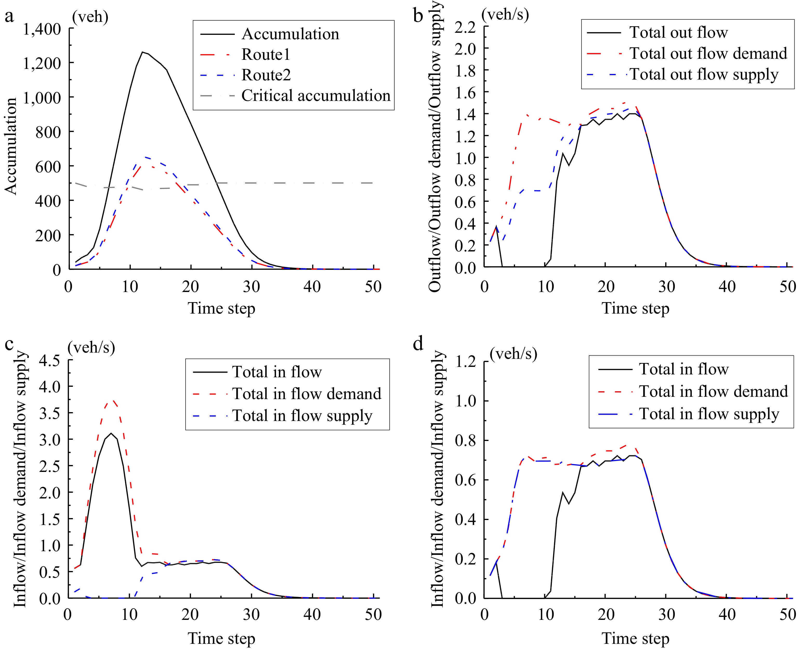
Figure 5.
Traffic dynamics. (a) Evolution of car accumulation in Reservoir 1. (b) Evolution of outflow in Reservoir 1. (c) Evolution of inflow in Reservoir 2. (d) Evolution of inflow in Reservoir 4.
Figure 5c & d display the inflow evolution in Reservoir 2 and Reservoir 4. The black, red and blue curves correspond to the effective inflow, inflow demand and inflow supply respectively. Note that we do not take into account the queue at the reservoir entrance. Because of the generation of travel demand in Reservoir 2 without any constraints, in Fig. 5c we can observe that there is an inflow greater than inflow supply. Since only transfer flow exists in Reservoir 4, inflow will not be greater than that of inflow supply. When the congestion disappears, its inflow supply will gradually increase, which will give more space for cars to enter this reservoir.
Based on the 3D-MFD, the bus speed in different reservoirs can be obtained under the condition that the accumulation of cars and buses are known. We can observe the bus speed evolution in Fig. 6a.
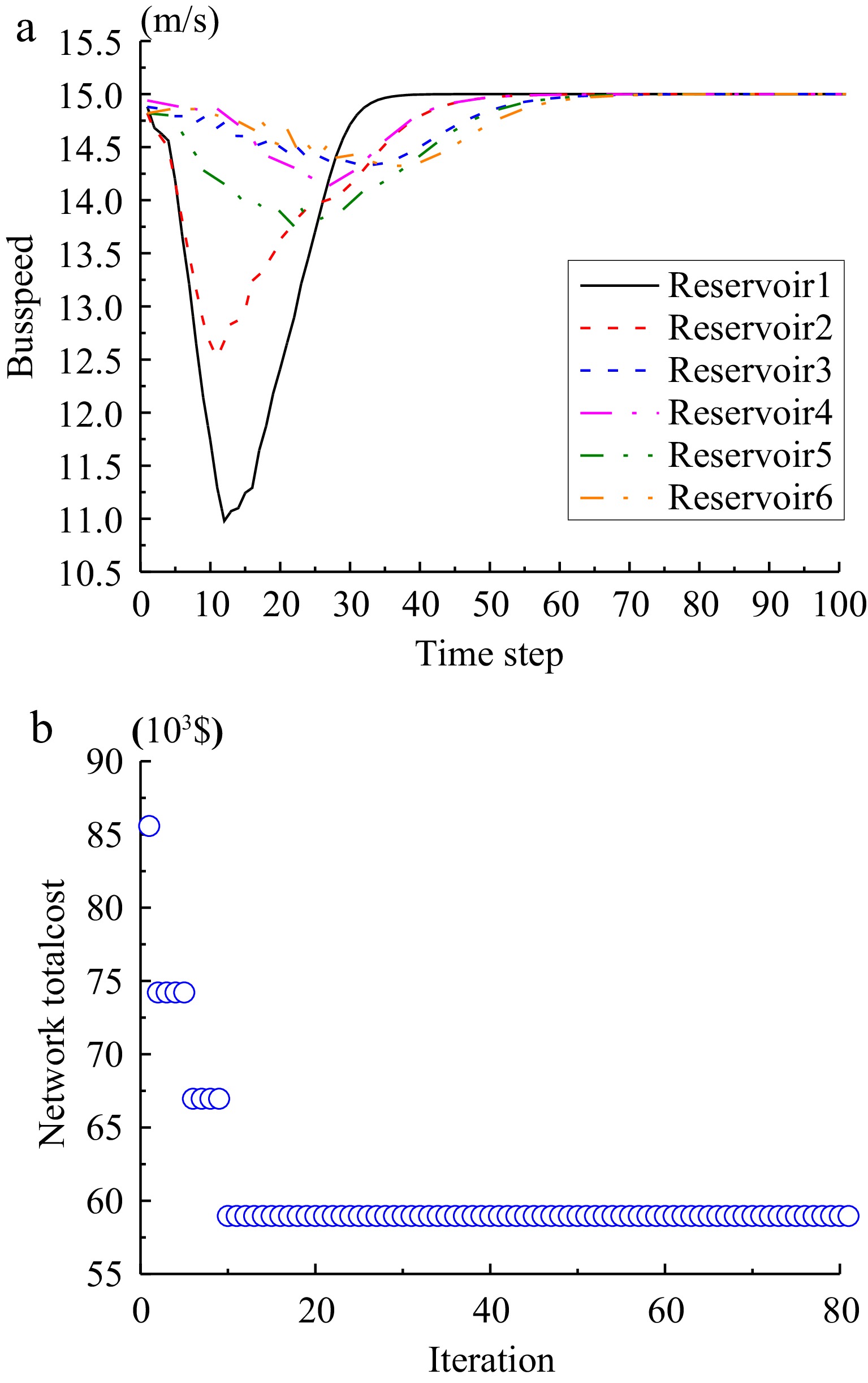
Figure 6.
Results on the (a) bus speed evolution and (b) convergence of the surrogate model based algorithm.
We display the dynamic path and mode choices of passengers, and the traffic flow evolution model of multi-reservoir can reproduce the traffic dynamics. It can be seen from Yildirimoglu & Geroliminis[34] that the evolution of congestion predicted by the MFD-based model is consistent with the micro-simulation results, Therefore, the model can predict the effect of route guidance strategy and congestion propagation in a large urban network.
Bus frequency optimization results
Convergence process of surrogate model-based algorithm
-
We use the surrogate model-based algorithm to solve the bi-level model, the algorithm can reach convergence when iterating to the 10th generation (see Fig. 6b).
Effect of considering 3D-MFD and dynamic user equilibrium
-
We compared different simulation results using 2D-MFD and 3D-MFD (Scenario 2 and Scenario 4). The total time spent of passenger and operating cost using 2D-MFD and 3D-MFD respectively are shown in Table 2.
Table 2. Total travel time of passengers and operation cost using 3D-MFD and 2D-MFD respectively.
Simulation 3D-MFD 2D-MFD The optimal frequency (min) {3.0, 4.0, 4.0, 3.0} {4.0, 0.2, 2.0, 1.0} Total time spent (veh·min) 106088.75 93111.93 Operation cost (${\$}$) 11700 44400 The objective value (${\$}$) 58894.38 68755.96 As shown in Table 2, without considering the complex interactions between buses and cars, the optimal frequency of buses is
$ \left\{\text{4}\text{.0},\text{0}\text{.2},\text{2}\text{.0},\text{1}\text{.0}\right\}\mathrm{min} $ ${\$} $ Then we analyze the results of equilibrium and non-equilibrium conditions using 3D-MFD based model (Scenario 3 and Scenario 4). That is to say, the path demand is known, and the influence of bus frequency optimization on travelers' path choices is not considered. We assume a simple case, that is, all the demands are distributed on each path. First, we analyze the difference optimal solution and objective value between the equilibrium type and non-equilibrium type of assignment models. The simulation results are shown in Table 3. The impact of bus frequency optimization on dynamic traffic assignment will be discussed later. Assuming that the optimal frequency is
$ \left\{\text{3}\text{.0},\;\text{4}\text{.0},\;\text{4}\text{.0},\;\text{3}\text{.0}\right\}\mathrm{min} $ ${\$} $ ${\$} $ Table 3. The optimal solution under equilibrium and non-equilibrium type.
Simulation Equilibrium Non-equilibrium Total time spent (veh·min) 106088.75 177269.47 Operation cost (min) 11700 35400 The objective value $\left( {\$} \right)$ 58894.38 106334.73 Under non-equilibrium conditions, the total travel time of the whole network system is obviously larger than the total time spent with scenario 2.
We also analyze the impact of varying the weight of total time spent on the studied system. In Fig. 7, we demonstrate how the weight of total time spent affects the delays and bus operation cost. As the weight (α) increases, , the total time spent decreases while the bus operation cost increases. Figure 8 depicts that the number of people opting for bus transportation increases as the weight (α) of total time spent increases. This suggests that we can encourage a shift towards bus travel by increasing the weight (α).
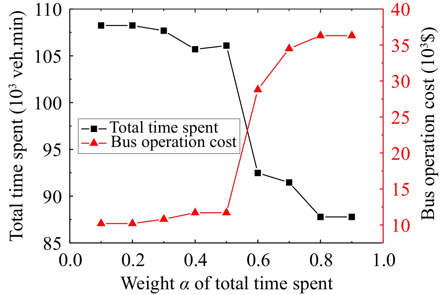
Figure 7.
Changes in the total time spent and bus operation cost for different weight values (α).
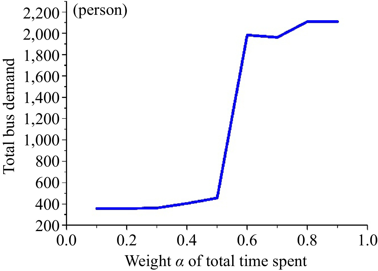
Figure 8.
The influence of the total time spent on the demand for bus travel.
Furthermore, we summarize the results of the optimal solution in 4 scenarios: 2D-MFD and 3D-MFD based models are considered under equilibrium and non-equilibrium conditions respectively. We denote
${Z_{\text{i}}}$ $i$ $\Delta {Z_{\text{i}}} = \left[ {{Z_{\text{i}}} - {Z_{\text{4}}}} \right]/{Z_{\text{4}}}$ Table 4. Comparison of the results of the optimal solution in 4 scenarios.
Simulation The optimal
frequency (min)The objective value ($ {\$} $) $\Delta {Z_{\text{i} } }$ (%) Scenario 1
(2D-MFD non-equilibrium){1.0, 0.5, 0.5, 0.5} 68,544.698 16.39 Scenario 2
(2D-MFD equilibrium){4.0, 0.2, 2.0, 1.0} 68,755.964 16.74 Scenario 3
(3D-MFD non-equilibrium){1.0, 0.5, 1.0, 1.0} 65,623.043 11.42 Scenario 4
(3D-MFD equilibrium){3.0, 4.0, 4.0, 3.0} 58,894.376 − In this paper, the dynamic traffic assignment model based on the 3D-MFD framework is used in the bi-level programming model to find the optimal bus frequency, that is, the bus departure interval is longer than other scenarios, seeing in Table 4, which will increase the waiting time of bus passengers, but in general, the upper level cost is smaller. The proposed bus frequency model integrating 3D-MFD and dynamic traffic assignment can achieve the best optimization results. The results reveal the value of the proposed model. And this new understanding of urban traffic network capacity is very important for formulating new strategies to improve traffic. In the future, we can integrate real-time traffic information or change the bus frequency to significantly improve the network performance.
-
We propose a bus frequency optimization framework, which considers impacts of traffic dynamics and travel mode choices. We formulate the bus frequency optimization problem as a bi-level programming problem. The upper-level problem minimizes the total time spent of passengers and bus operation cost. To achieve this, we incorporate a region-based dynamic traffic assignment model and a 3D-MFD based dynamics network loading model as the lower-level problem. Travelers determine their mode choices based on travel time, which is calculated using the network loading model. For bus travelers, the travel time comprises the time spent on roads and waiting at bus stops.
In the 3D-MFD based model, we utilize an accumulation-based model to represent car traffic dynamics, while a trip-based model is used for bus dynamics. The accumulation of buses determines an MFD, which relates the average car speed (and the outflow) to the accumulation of cars. The bus speed is dependent on the accumulation of both buses and cars. Whenever a trip distance is completed within a reservoir, the bus exits that reservoir.
To optimize computation time, we employ a double projection algorithm for solving the lower-level multi-modal DUE problem. Additionally, we have developed a surrogate model-based algorithm to solve the proposed bi-level programming problem.
By incorporating these techniques, our framework offers a novel approach to bus frequency optimization that considers traffic dynamics and travel mode choices. Numerical results display the convergence result of two algorithms and the evolution of speed and accumulation in the reservoirs. We also study the bus frequency setting problem in case of multi-modal traffic networks and analyze the influence of the optimal frequency when the weight of passenger total time spent and that of bus operator's cost are changed. Then, we analyze the different optimization results between the 2D-MFD and 3D-MFD based models and equilibrium type and non-equilibrium type of assignment models. Finally, we compare the results of the optimal solution in four scenarios: 2D-MFD and 3D-MFD based model are considered under equilibrium and non-equilibrium conditions respectively. The results reveal the value of considering multimodal interactions and dynamic user equilibrium. This optimization framework ensures that determined bus frequency actually leads to efficient bus service in the transit network.
Promoting modal shift towards public transport, particularly buses, while minimizing the total delays of all travelers, remains a significant research question in practical implementation. To encourage modal shift towards public transport, we propose a bus frequency optimization framework that focuses on improving bus operations. Our model incorporates Dynamic Traffic Assignment (DTA) to analyze modal choices, enabling us to assess the impact of bus operations on the demand distribution between buses and cars. A model without DTA would underestimate the impacts of bus operation on the modal shift and its impacts on the road traffic system.
The proposed framework can be extended to a transportation system with a subway. The extension with a subway is in a straightforward way because it only affects the mode choices. To handle the large-scale problem, this work treats the studied city as a multi-reservoir system. To implement this aggregation approach in real life, we still need to address many other research questions, which would be the future research direction. We propose three research directions: (i) In each reservoir, several bus stops are aggregated as one virtual bus stop. An optimization approach to aggregate these bus stops is required. (ii) We assume the regional average trip length for cars is constant. But regional trip lengths vary over time[34]. We will further study the impact of heterogeneity of trip length on optimal bus frequency. (iii) The calibration and verification of the model and the algorithms would also need more effort.
-
The authors confirm contribution to the paper as follows: study conception and design: Long J; analysis and interpretation of results: Cui D, Long J, and Yuan K; draft manuscript preparation: Yuan K, Cui D, and Long J. All authors reviewed the results and approved the final version of the manuscript.
-
Data sharing not applicable to this article as no datasets were generated or analyzed during the current study.
This work is jointly supported by the National Natural Science Foundation of China (Grant No. 72201088, 71871077, 71925001), the Fundamental Research Funds for the Central Universities of China (Grant No. PA2022GDSK0040, JZ2023YQTD0073), which are gratefully acknowledged.
-
The authors declare that they have no conflict of interest. Jiancheng Long is the Editorial Board member of Digital Transportation and Safety. He was blinded from reviewing or making decisions on the manuscript. The article was subject to the journal’s standard procedures, with peer-review handled independently of this Editorial Board member and the research groups.
- Copyright: © 2023 by the author(s). Published by Maximum Academic Press, Fayetteville, GA. This article is an open access article distributed under Creative Commons Attribution License (CC BY 4.0), visit https://creativecommons.org/licenses/by/4.0/.
-
About this article
Cite this article
Yuan K, Cui D, Long J. 2023. Bus frequency optimization in a large-scale multi-modal transportation system: integrating 3D-MFD and dynamic traffic assignment. Digital Transportation and Safety 2(4):241−252 doi: 10.48130/DTS-2023-0020 

Bus frequency optimization in a large-scale multi-modal transportation system: integrating 3D-MFD and dynamic traffic assignment
- Received: 25 June 2023
- Accepted: 07 October 2023
- Published online: 28 December 2023
Abstract: A properly designed public transport system is expected to improve traffic efficiency. A high-frequency bus service would decrease the waiting time for passengers, but the interaction between buses and cars might result in more serious congestion. On the other hand, a low-frequency bus service would increase the waiting time for passengers and would not reduce the use of private cars. It is important to strike a balance between high and low frequencies in order to minimize the total delays for all road users. It is critical to formulate the impacts of bus frequency on congestion dynamics and mode choices. However, as far as the authors know, most proposed bus frequency optimization formulations are based on static demand and the Bureau of Public Roads function, and do not properly consider the congestion dynamics and their impacts on mode choices. To fill this gap, this paper proposes a bi-level optimization model. A three-dimensional Macroscopic Fundamental Diagram based modeling approach is developed to capture the bi-modal congestion dynamics. A variational inequality model for the user equilibrium in mode choices is presented and solved using a double projection algorithm. A surrogate model-based algorithm is used to solve the bi-level programming problem.