-
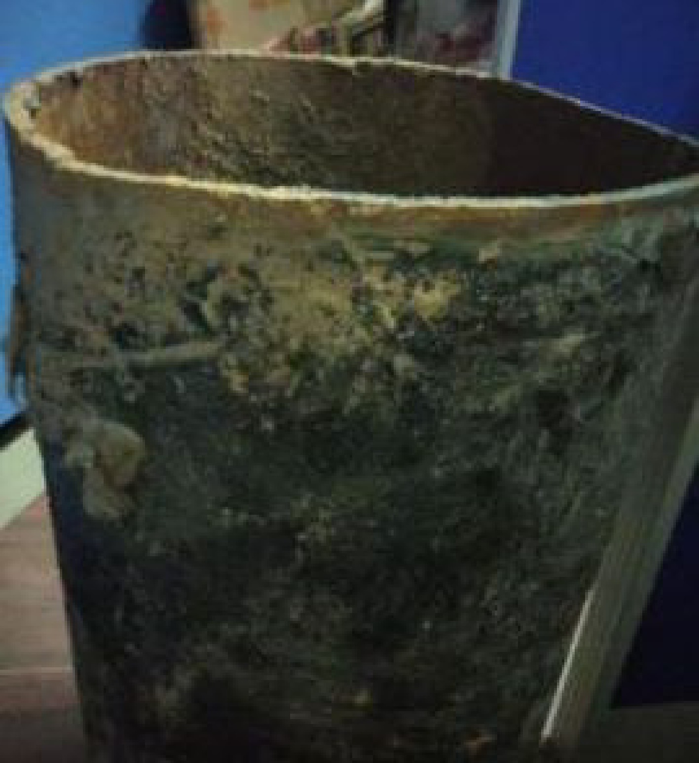
Figure 1.
Pipeline corrosion sample.
-
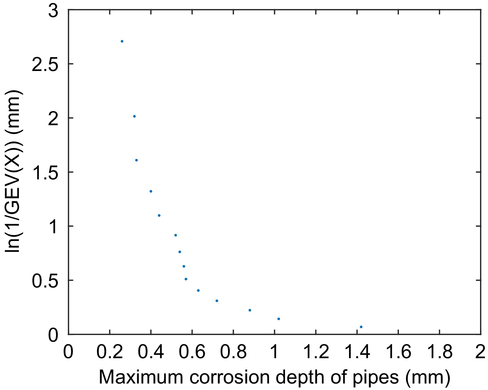
Figure 2.
Cumulative probability distribution law of local maximum corrosion depth of the pipeline.
-
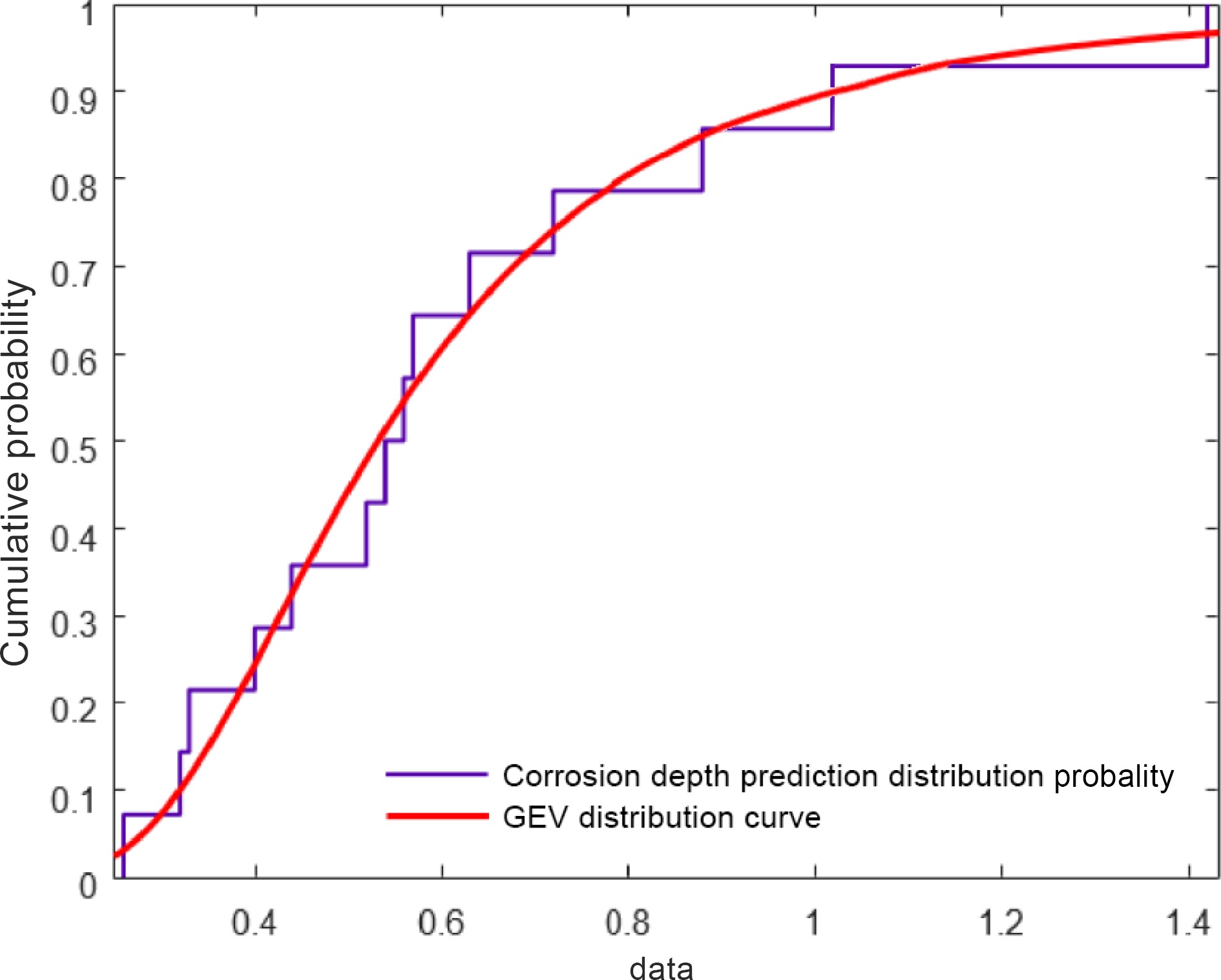
Figure 3.
Probability distribution curve of corrosion depth.
-
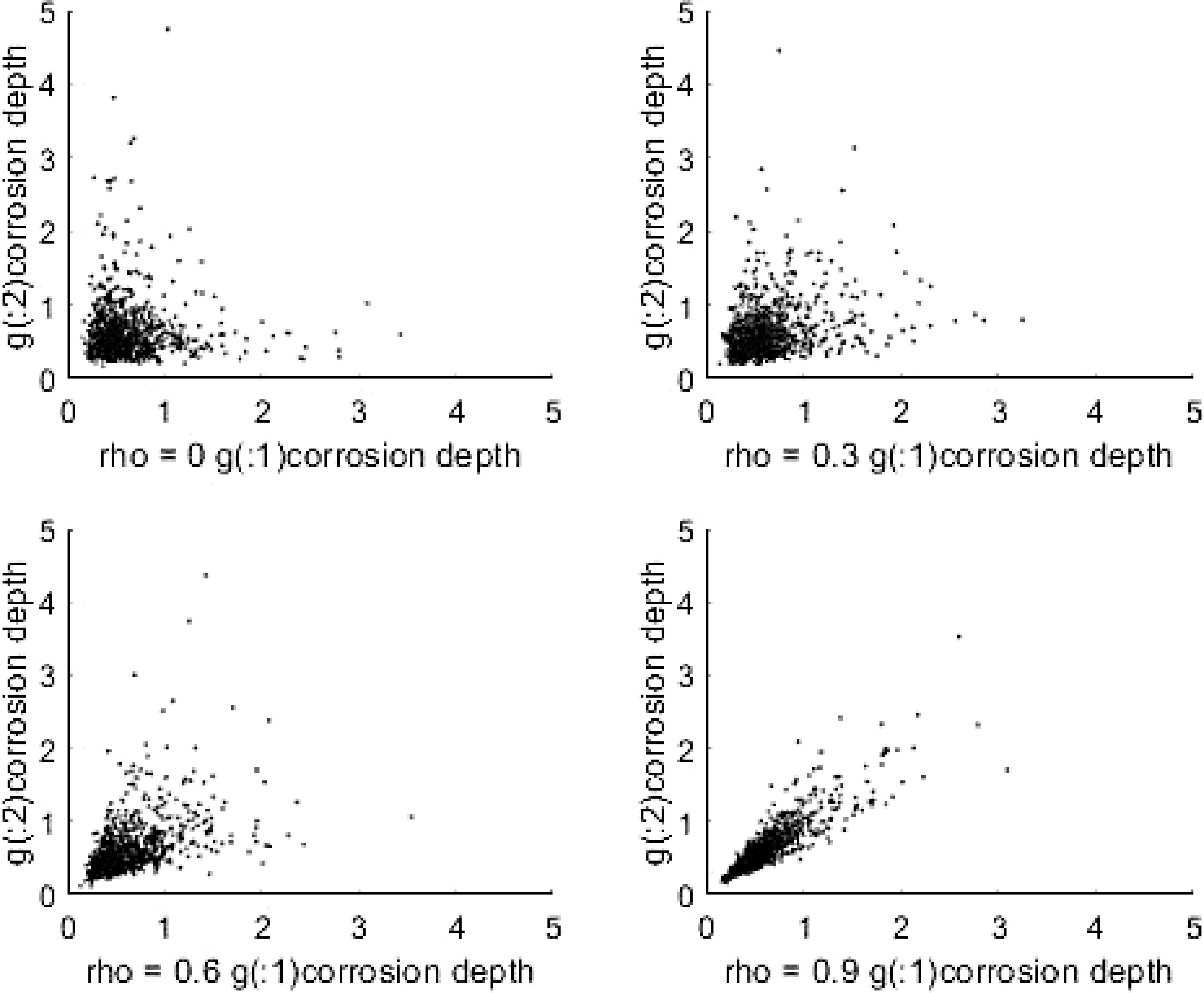
Figure 4.
Distribution of corrosion depth under different correlation coefficients.
-
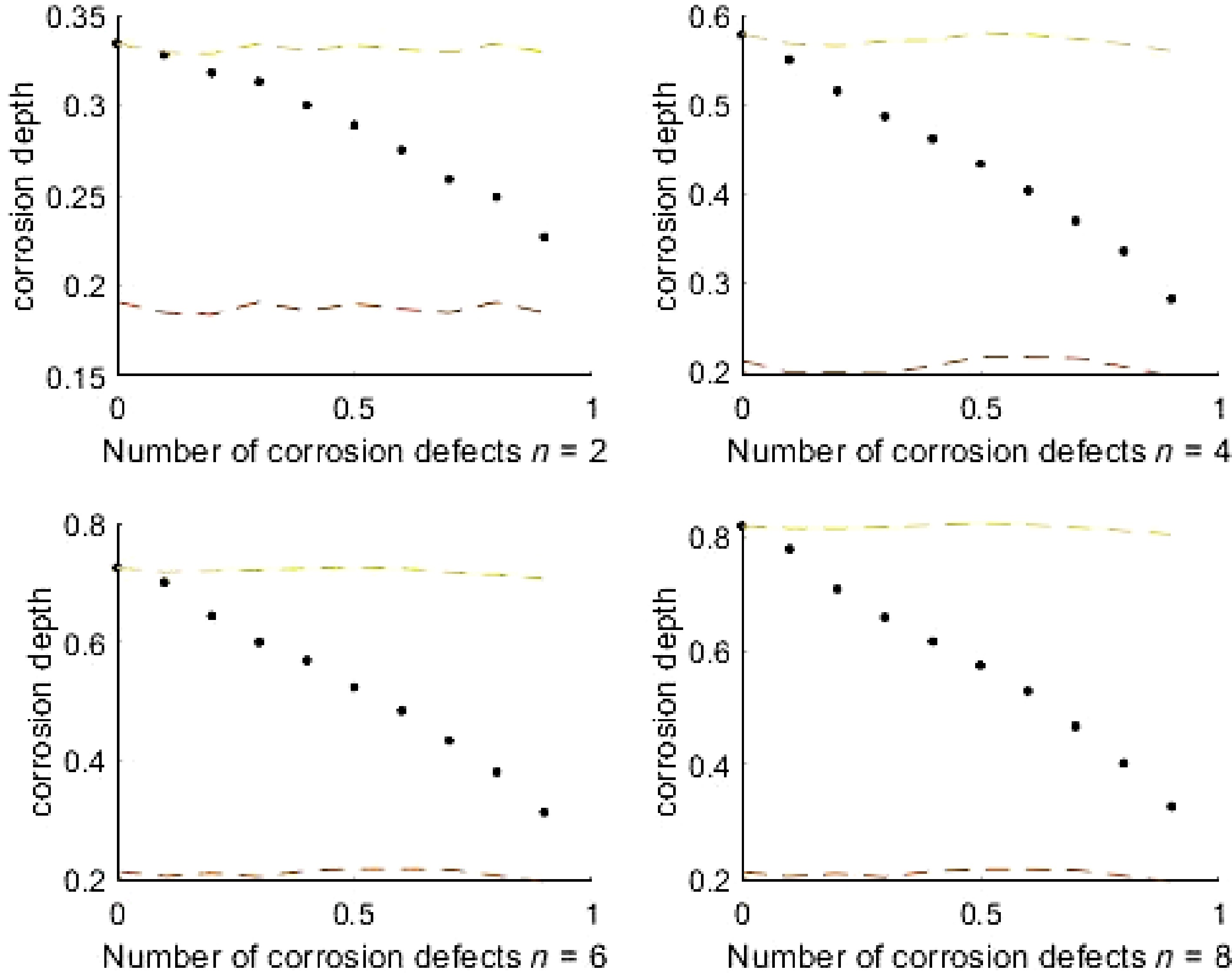
Figure 5.
Trend diagram of system failure probability with correlation coefficient of pipeline corrosion defects.
-
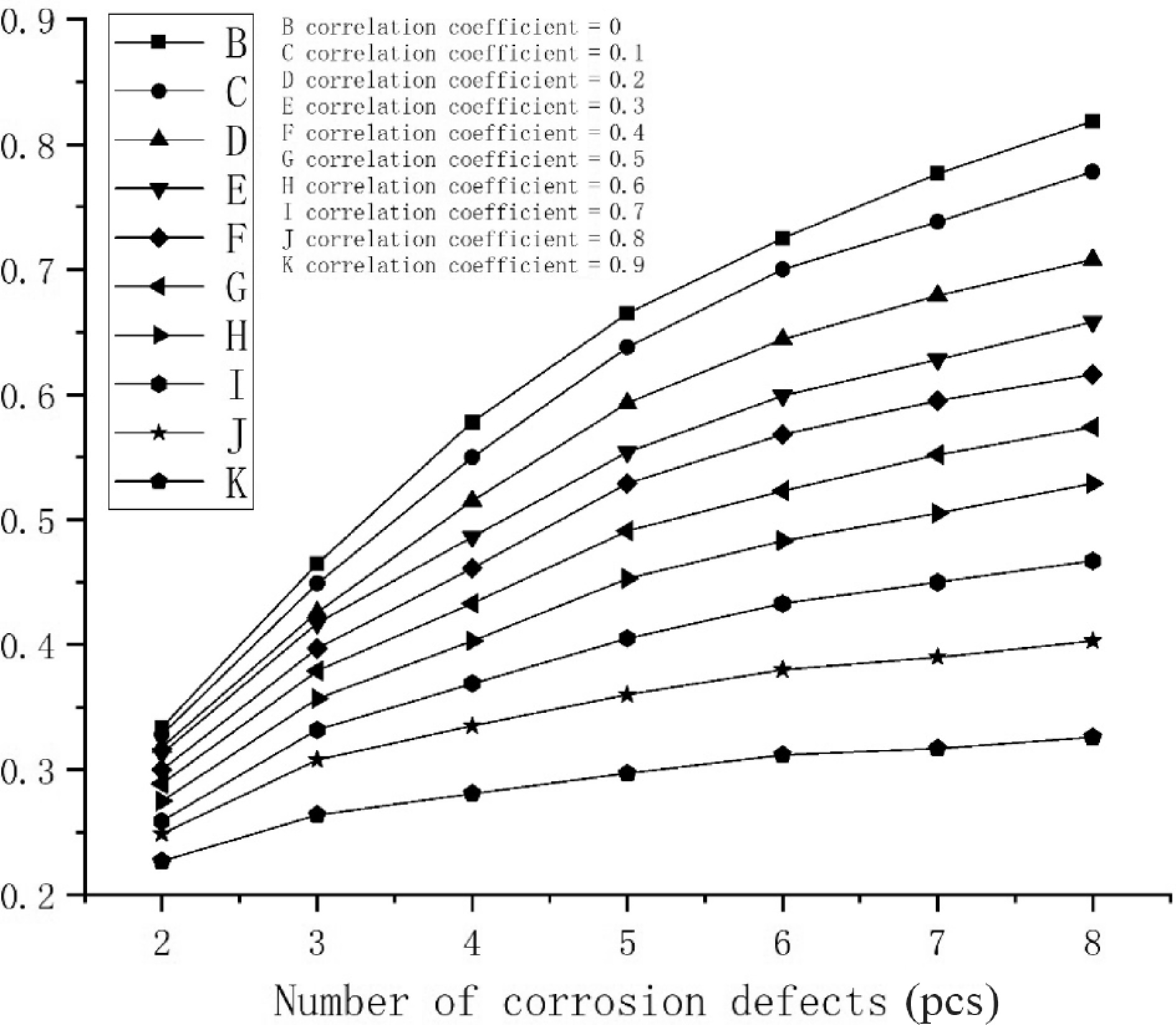
Figure 6.
Trend diagram of system failure probability with pipeline corrosion defects.
-
Parameter Average value Variable coefficient Unit Distribution form Axial length of corrosion defect (L) 30 35% mm Logarithmic normal distribution Outer diameter (d) 60 1% mm Normal distribution Maximum annual internal pressure (p) 0.259 − Mpa Definite value Thickness (t) 4 1.5% mm Normal distribution Yield strength $ ({\mathit{\sigma }}_{\mathit{u}} $ 235 3% Mpa Normal distribution Accuracy coefficient of model ( $ {\mathit{x}}_{\mathit{m}} $ 0.97 10.5% − Normal distribution Table 1.
Pipeline parameters and probability distribution form.
-
Sample number Residual pipe wall thickness (mm) Sample number Residual pipe wall thickness (mm) 1 3.12 8 3.56 2 3.48 9 3.43 3 3.67 10 2.58 4 3.60 11 3.28 5 3.46 12 2.98 6 3.74 13 3.37 7 3.68 14 3.44 Table 2.
Residual wall thickness of pipeline.
Figures
(6)
Tables
(2)