


-
Affected by the external environment such as soil medium, stray current, and microbial corrosion, external corrosion (mostly localized corrosion) often occurs in gas pipelines during service; accidents such as fire and explosion occur. Therefore, characterizing the uncertainty distribution of corrosion defects and propagating this uncertainty into the failure probability prediction model is crucial for formulating the maintenance cycle and improving the reliability of the pipeline.
Jia[1], Xi[2] and other scholars studied the application of the generalized extreme value distribution model in the characteristics of corrosion defect probability distribution. Taking the soil corrosion test data of Tarim and Dagang oil fields as an example, Weng[3] demonstrated that the overall probability distribution of the regional corrosion test data conforms to the normal random function and the maximum data conforms to the Gumbel function. The statistical results show that the Gumbel function can be used to describe the probability distribution of the maximum corrosion depth of pipelines in the short term. The probability distribution of the maximum corrosion depth of the pipeline changes with different service time. However, in most pipeline failure probability calculation studies, each corrosion defect of the pipeline is regarded as an independent event affecting pipeline failure, and the events are independent of each other, and then the series model is used to calculate the failure probability of the pipeline. Since the soil and other external environment around the adjacent defects have similar corrosion characteristics with the pipeline, the random growth of these defects may be correlated, and the results obtained by using the series model are different from the actual situation. This correlation should be taken into account when evaluating the system reliability of natural gas pipelines with multiple corrosion defects and developing appropriate failure prevention measures. Yu[4] proved that the binary copula function can be constructed and applied to practical problems based on the correlation between the data. Wang et al. and Zhang et al.[5,6] considered copula function to predict pipeline corrosion defects. Based on this, Zeng[7] proposed a calculation method of pipeline failure probability based on correlation coefficient theory to simulate the correlation between corrosion defects, which can accurately evaluate the reliability of pipeline system. In order to evaluate the reliability of a pipeline system with multiple corrosion defects, the generalized extreme value distribution model (GEV) can be used as a suitable model to describe the maximum depth of corrosion, while the Copula-based method can reasonably simulate the random correlation between the growth of different defects.
-
The research shows that the probability distribution of the maximum corrosion depth of the pipeline varies with the actual situation. The limitation of a single extreme value distribution type will lead to the low prediction accuracy of the built model, while the GEV distribution can adaptively optimize the extreme value distribution according to the simulated parameters. GEV distribution is the probability distribution of the maximum value (minimum value) set in probability theory, let
$ y=\dfrac{x-\mu }{\sigma } $ Gumbel distribution (
$ \eta =0 $ $ {F}_{1}\left(y\right)=\mathit{exp}(-\mathit{exp}(-y\left)\right),\forall y $ (1) Frechet distribution (
$ \eta > 0 $ $ {F}_{2}\left(y\right)=\left\{\begin{array}{cc}0,& y\le 0\\ \mathit{exp}(-{y}^{-\eta }),& y \gt 0\end{array}\right. $ (2) Weibull distribution (
$ \eta < 0 $ $ {F}_{3}\left(y\right)=\left\{\begin{array}{cc}\mathit{exp}(-{y}^{-\eta }),& y\le 0\\ 1,& y \gt 0\end{array}\right. $ (3) $ x $ $ \mu $ $ \sigma $ $ \eta $ From Eqns (1) to (3), the cumulative probability distribution function of the GEV distribution can be deduced:
$ \text{GEV(}x)=\mathit{exp}(-(1+\eta y{)}^{-1/\eta }),\;\; 1+\eta y \gt 0 $ (4) Copula function
-
The Copula function is the joint distribution function of n (n ≥ 2) standard uniformly distributed variables
$ {U}_{i} $ $ \mathrm{C}({\mathrm{u}}_{1},\,{\mathrm{u}}_{2},\,...,\,{\mathrm{u}}_{\mathrm{n}})=\mathrm{P}({\mathrm{U}}_{1} \lt {\mathrm{u}}_{1},\, {\mathrm{U}}_{2} \lt {\mathrm{u}}_{2},\, ...,\, {\mathrm{U}}_{\mathrm{n}} \lt {\mathrm{u}}_{\mathrm{n}}) $ (5) $ C({u}_{1},\,{u}_{2},\,...,\,{u}_{n}) $ $ {u}_{i} $ $ {U}_{i} $ $ \mathrm{C}\left({\mathrm{F}}_{1}\right({\mathrm{x}}_{1}),\,{\text{F}}_{2}({\mathrm{x}}_{2}),\,...,\,{\text{F}}_{\mathrm{n}}({\mathrm{x}}_{\mathrm{n}}\left)\right)=\mathrm{F}({\mathrm{x}}_{1},\,{\mathrm{x}}_{2},\,...,\,{\mathrm{x}}_{\mathrm{n}}) $ (6) In the formula, Fi(xi), i = 1, 2, ..., n is the marginal probability distribution function of F(x1, x2, ..., xn). In addition, with the parameter Fi(xi),the copula is a function with marginal distribution Fi(xi) multivariate distribution function. Copula function set includes Gaussian Copula function, T-Copula function and Gumbel Copula function. In this study, Gaussian copula was selected to characterize the correlation between different corrosion defects.
$ \mathrm{C}({\mathrm{u}}_{1},\,{\mathrm{u}}_{2},\,...,\,{\mathrm{u}}_{\mathrm{n}})={\mathrm{\Phi }}_{\mathrm{n}}({\mathrm{\Phi }}^{-1}({\mathrm{u}}_{1}),\,{\mathrm{\Phi }}^{-1}({\mathrm{u}}_{2}),\,...,\,{\mathrm{\Phi }}^{-1}({\mathrm{u}}_{\mathrm{n}});\;\mathrm{R}) $ (7) $ {\Phi }_{n}(;\;R) $ $ {\Phi }^{-1}\left(\right) $ -
Since it is difficult to obtain the data of the entire pipeline, this paper adopts the method of estimating a large sample with a small sample, and conducts sampling detection to obtain the data in the most severely corroded area.
If the distribution law of pipeline corrosion depth is to be verified by imaging, it may be assumed that n samples of corroded pipelines are drawn, and the maximum corrosion depth xi (i = 1, 2, …, n) of each area is used as a statistical variable, and then sorted from big to small, and then the average permutation method of sequential statistics is used to calculate the cumulative probability, which is:
$ \text{GEV(}{\mathrm{x}}_{\mathrm{i}})=\dfrac{\mathrm{i}}{\mathrm{n}+1},\quad\quad \mathrm{n}=\mathrm{1,2},...,\mathrm{n} $ (8) n = 1, 2, ..., n,Fitting xi and
$ \text{ln(1/GEV(}{x}_{i}\left)\right) $ Based on the MATLAB program, the GEV distribution parameters were fitted to obtain the corresponding
$ \mu $ $ \sigma $ $ \eta $ Failure modes and limit state equations of pipelines
-
The limit state function (LSF) can be used to define the corresponding failure mode, on the basis of which appropriate maintenance measures can be taken. This article uses two limit state functions to define small leaks and bursts. A small leak is defined as a failure event in which a defect (i.e., corrosion pit) penetrates a pipe wall to its wall thickness threshold percentage. Based on industry practice, a wall thickness threshold of 80% is recommended. Therefore, the first limit state function is:
$\\{\mathrm{LSF}}_{1}={\mathrm{0.2}}{\mathrm t}-{\mathrm{d}} $ (9) Where, d is the corrosion depth of the pipeline.
For bursting, its limit state function is:
$ {\mathrm{L}\mathrm{S}\mathrm{F}}_{2}={\mathrm{P}}_{\mathrm{b}}-{\mathrm{P}}_{\mathrm{o}\mathrm{p}} $ (10) Where is the pipeline operating pressure, its commonly used models include improved B31G, PCORRC, DNV-RPF10 and other methods. In this paper, we use the improved B31G model to calculate the burst pressure, and its calculation formula is as follows:
$ {\mathrm{P}}_{\mathrm{b}}=\mathrm{\lambda }\dfrac{2\mathrm{t}}{\mathrm{D}}\mathrm{\sigma }\left[\dfrac{1-0.85\dfrac{\mathrm{d}}{\mathrm{t}}}{1-0.85\dfrac{\mathrm{d}}{\mathrm{t}}\dfrac{1}{\mathrm{M}}}\right] $ (11) $ \left\{\begin{array}{l}M=\sqrt{1+\text{0.6275}\left(\dfrac{\text{2L}}{\sqrt{Dt}}\right)^{2}-0.003375\left(\dfrac{\text{2L}}{\sqrt{Dt}}\right)^{4}},\;L\le \sqrt{50Dt}\\ M=3.3+0.032\left(\dfrac{L}{\sqrt{Dt}}\right)^{2},\;L \gt \sqrt{50Dt}\end{array}\right. $ (12) Pb is the pipe failure pressure (Mpa); L is the axial corrosion length, mm; λ is the error factor of multiplication model; D is the pipe outer diameter, mm; σ is the yield strength (Mpa); d is the corrosion depth of the pipeline, mm; t is the pipe wall thickness, mm; M is Folias expansion coefficients.
By LSF1, LSF2, small leakage can be defined as
$ LS{F}_{1}\le 0\;\cap LS{F}_{2} > 0 $ $ LS{F}_{1} > 0\cap LS{F}_{2}\le 0 $ Calculation of system failure probability of the pipeline
-
The Stevnson-Moses method is a typical point estimation method. Its core idea is to assume that the mutual relationship between the failure modes in the series system is two ideal states, such as complete positive correlation or mutual independence. The failure modes of the structural system are not completely positively correlated with each other, nor are they completely independent, so the results obtained by the Stevnson-Moses algorithm tend to be conservative or unsafe. Suppose the system failure probability of a pipeline with corrosion defects is Pf, then there are:
$ \text{max}{\text{P}}_{{\mathrm{f}}_{\mathrm{i}}}\le {\mathrm{P}}_{\mathrm{f}}\le 1-{\prod }_{\mathrm{i}=1}^{\mathrm{i}}\;(1-{\text{P}}_{{\mathrm{f}}_{\mathrm{i}}}) $ (13) $ {P}_{{f}_{i}} $ It can be seen that the Stevnson-Moses method can only describe the range of system failure probability. This paper proposes a system failure probability analysis method based on Monte Carlo simulation, which can accurately calculate the actual system failure of pipelines containing multiple corrosion defects probability, the calculation steps are as follows:
1) Let N0 = 0, SL = 0, SL represents the number of leaks in the pipeline;
2) According to the distribution model of corresponding variables, generate random variables or fixed value samples such as wall thickness, pipe outer diameter and tensile strength;
3) n (n = 2, 4, 6, 8, 10) pieces of corrosion depth data with correlation coefficients of 0, 0.1, ..., 0.9 are respectively generated by the Copula function;
4) The value of LSF1, LSF2 is calculated according to the corresponding variable,
5) If LSF1 ≤ 0, so that SL = SL+1;
6) Let N0 = N0 + 1; If N0 < N, stop the cycle.
For the total number of N simulation tests, the failure probability PSL of small leakage and rupture of the pipeline can be calculated by the following formula:
$ {\mathrm{P}}_{\mathrm{S}\mathrm{L}}\approx \dfrac{1}{\mathrm{N}}\mathrm{S}\mathrm{L} $ (14) -
The Nanjing gas transmission pipeline has a history of more than 40 years since the 1970s, and a large number of gas pipelines in the main urban area have been in service for more than 10 years. When the pipelines were excavated, it was found that the sample pipelines had multiple corrosion phenomena, as shown in Fig. 1. The surface of the pipeline has been corroded by soil, microorganisms and other environmental factors over a long period, and the surface pitting corrosion phenomenon is serious. The main form was local corrosion on the outside of the pipelines.
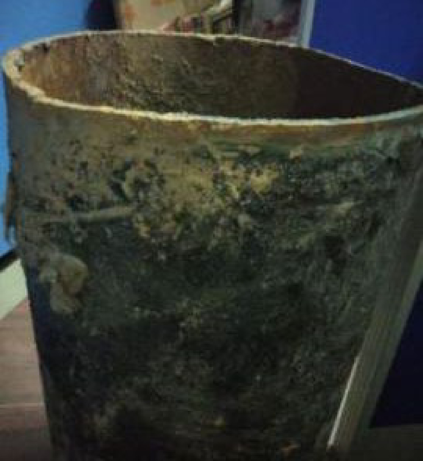
Figure 1.
Pipeline corrosion sample.
In this paper, a certain section of pipeline was selected for analysis, and the material is Q235 steel. The measured data are shown in Table 1.
Table 1. Pipeline parameters and probability distribution form.
Parameter Average value Variable coefficient Unit Distribution form Axial length of corrosion defect (L) 30 35% mm Logarithmic normal distribution Outer diameter (d) 60 1% mm Normal distribution Maximum annual internal pressure (p) 0.259 − Mpa Definite value Thickness (t) 4 1.5% mm Normal distribution Yield strength $ ({\mathit{\sigma }}_{\mathit{u}} $) 235 3% Mpa Normal distribution Accuracy coefficient of model ($ {\mathit{x}}_{\mathit{m}} $) 0.97 10.5% − Normal distribution Fourteen groups of pipeline sections with serious corrosion degree are selected, and the results of residual wall thickness of pipeline are the average values of five measurements, as shown in Table 2.
Table 2. Residual wall thickness of pipeline.
Sample number Residual pipe wall thickness (mm) Sample number Residual pipe wall thickness (mm) 1 3.12 8 3.56 2 3.48 9 3.43 3 3.67 10 2.58 4 3.60 11 3.28 5 3.46 12 2.98 6 3.74 13 3.37 7 3.68 14 3.44 Determination of GEV model parameters
-
Select the maximum corrosion depth of each section of pipeline, and calculate the GEV distribution probability of corrosion depth by the average arrangement method of sequential statistics. As shown in Fig. 2, the local maximum corrosion depth of pipeline xi and
$ {\text{ln(1/GEV}}({x_i})) $ 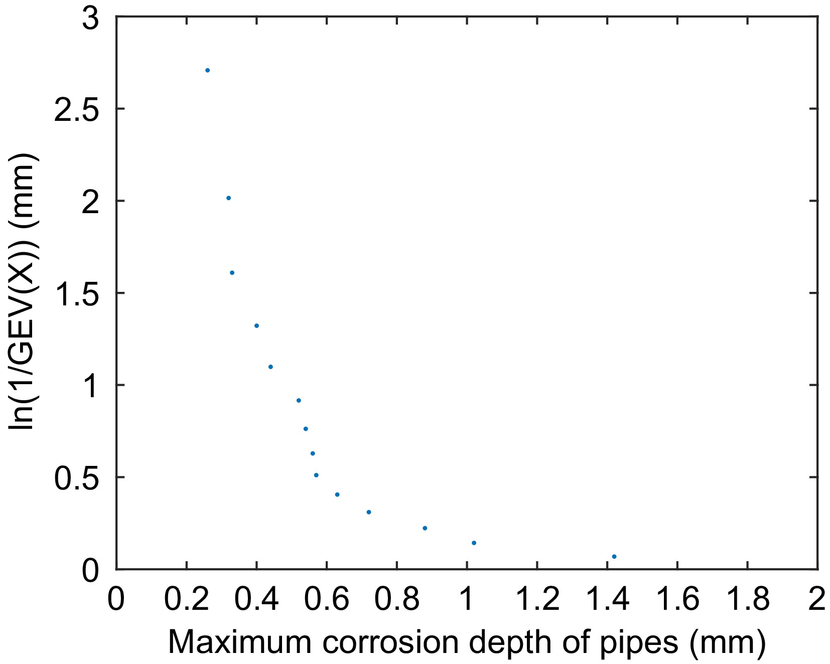
Figure 2.
Cumulative probability distribution law of local maximum corrosion depth of the pipeline.
The model parameters are fitted by MATLAB,
$ \eta $ $ \mu $ $ \sigma $ $ \eta $ 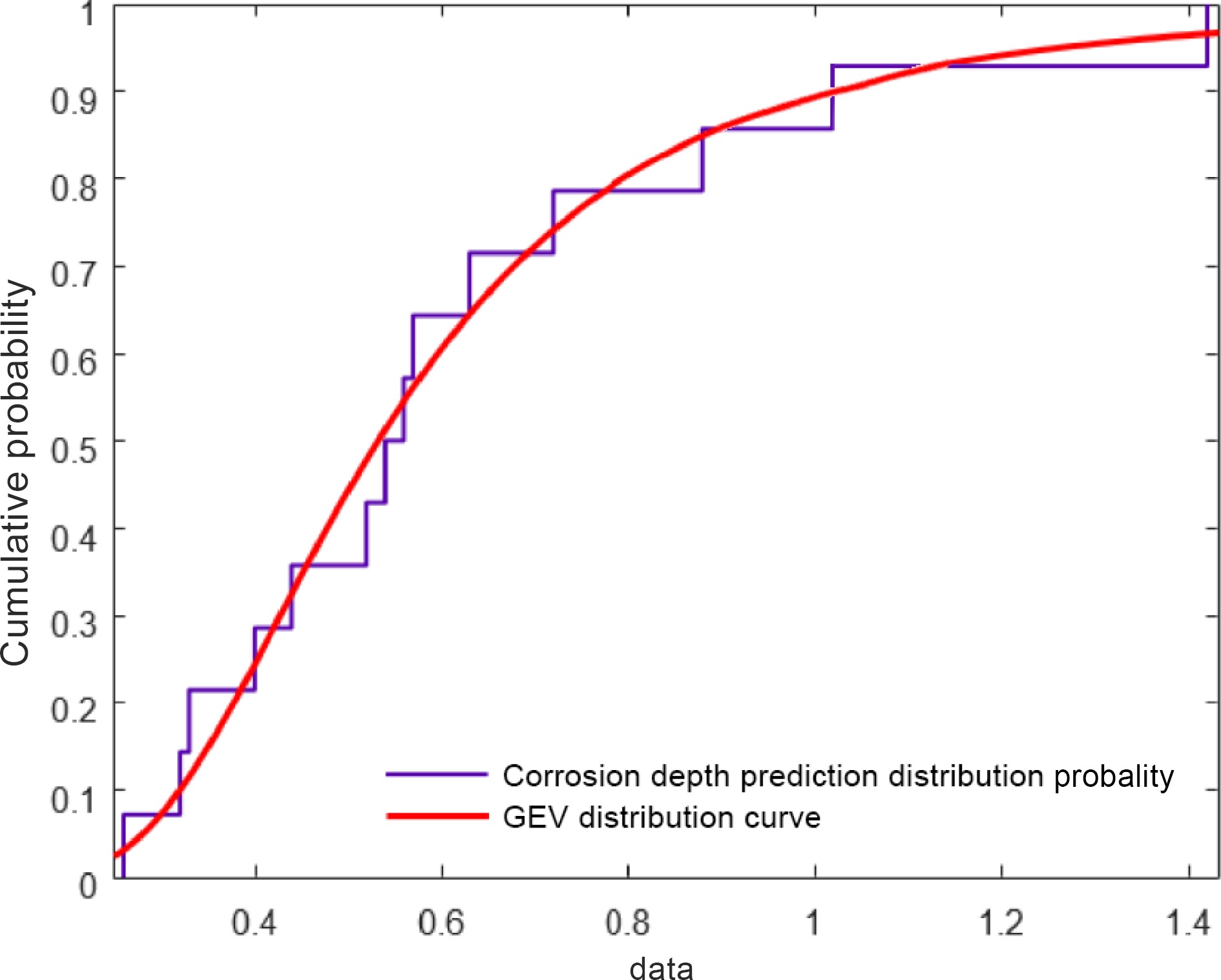
Figure 3.
Probability distribution curve of corrosion depth.
Simulation of pipeline corrosion depth under different correlation coefficients
-
The Copula function can be used to fit the depth data of pipeline corrosion defects with different correlation coefficients. To illustrate this method, 1,000 correlation coefficients (rho) are randomly generated. Two-dimensional pipeline corrosion depth data of 0, 0.3, 0.6 and 0.9, respectively, and their distributions are shown in Fig. 4.
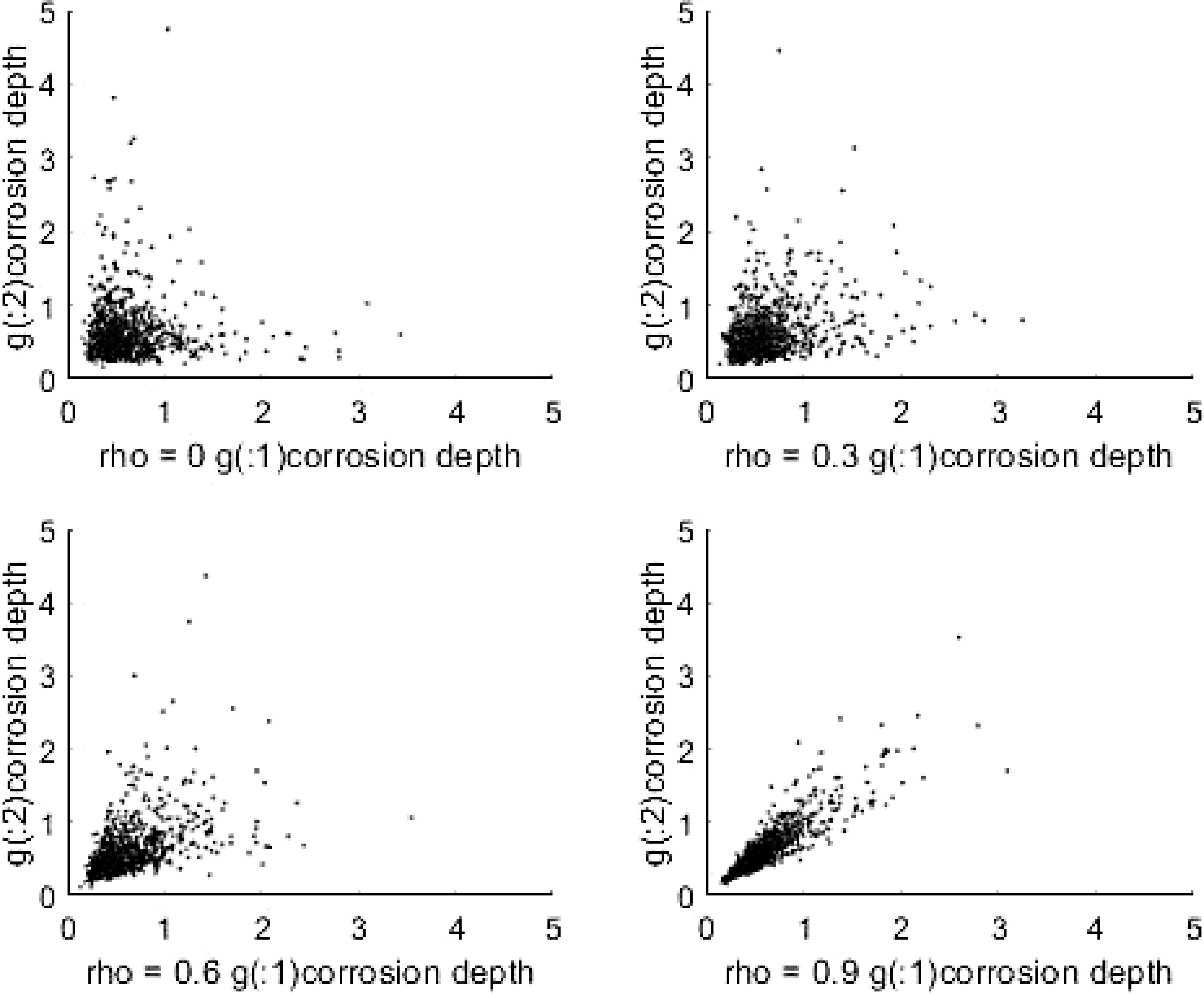
Figure 4.
Distribution of corrosion depth under different correlation coefficients.
It can be seen from Fig. 4 that as the correlation coefficient (rho) between the data increases, the corrosion depth distribution becomes more regular. When the correlation coefficient is 1, the two sets of corrosion depth data will be completely linear.
Calculation results and analysis of pipeline failure probability
-
Because the internal pressure of the pipeline is less than 25% yield strength, the pipeline is operated under low circumferential stress conditions, and the failure mode is perforation failure caused by corrosion. Therefore, the failure probability of pipeline system in this paper is the probability of small leakage. As is shown in Fig. 5, The corrosion depth decreases with the increase of correlation coefficient. The Fig. 6 shows the change trend of the system failure probability value of the pipeline with the increase of the correlation coefficient between corrosion defects when the number of pipeline corrosion defects is set as 2, 4, 6, and 8 respectively. As can be seen from the following figure, the system failure probability of the pipeline is within the upper and lower limits. Therefore, the failure probability calculation method adopted in this paper is effective.
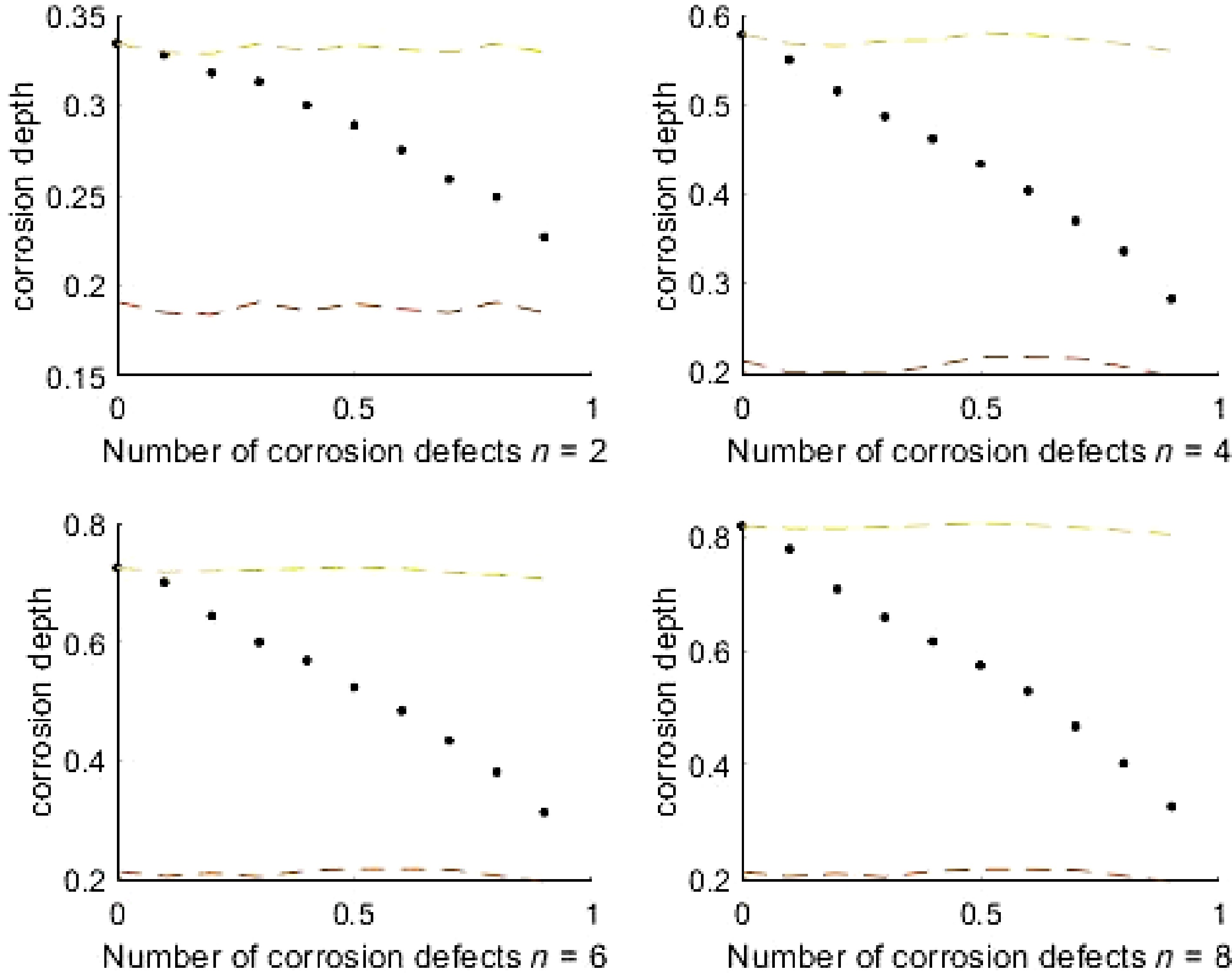
Figure 5.
Trend diagram of system failure probability with correlation coefficient of pipeline corrosion defects.
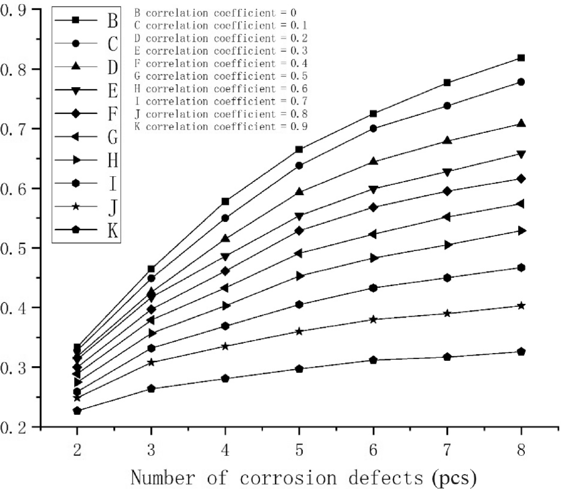
Figure 6.
Trend diagram of system failure probability with pipeline corrosion defects.
Generally speaking, the system failure probability of a pipeline decreases with the increase of correlation coefficient, because the larger the correlation coefficient, the greater the joint failure probability of corrosion defects. For example, for a pipeline with two corrosion defects, the system failure probability is Pf =
$ {{\text{P}}_{{{\text{f}}_1}}} \cup {\text{P}}{}_{{{\text{f}}_2}} $ $ {{\text{P}}_{{{\text{f}}_1}}}{\text{ + P}}{}_{{{\text{f}}_2}}{{ - }}\;{{\text{P}}_{{{\text{f}}_1}}} \cap {\text{P}}{}_{{{\text{f}}_2}} $ ${{\text{P}}_{{{\text{f}}_1}}} \cap {\text{P}}{}_{{{\text{f}}_2}}$ $ {{\text{P}}_{{{\text{f}}_1}}} $ $ {{\text{P}}_{{{\text{f}}_{\text{2}}}}} $ ${1-}{\displaystyle \prod _{\text{i}=1}^{\text{i}}({{1-{\rm P}}}_{{\text{f}}_{\text{i}}})} $ $ {1-}{\displaystyle \prod _{\text{i}=1}^{\text{i}}({{1-{\rm P}}}_{{\text{f}}_{\text{i}}})} $ The influence of the number of defects on the probability of pipeline failure is shown in Fig. 6. When the correlation coefficient is less than 0.6, the failure probability of the pipeline system fluctuates greatly with the increase of the number of corrosion defects. When the number of defects increases from 2 to 8, the pipeline failure probability increases by more than 100%. As the number of corrosion defects increases with the correlation of corrosion defects, the impact on the system failure probability becomes smaller.
-
In this paper, the GEV model is adopted, and the corresponding extreme value distribution model is selected according to the simulated parameters. Through graphic verification and MATLAB software data fitting, it can be concluded that the threshold parameters
$ \eta $ The method used in this paper calculates that the pipeline failure probability falls within the upper and lower limits of Stevnson-Moses method, indicating that the pipeline corrosion probability calculation method adopted in this paper is effective and reliable when defects are correlated.
The system failure probability of the pipeline decreases with the increase of the correlation coefficient, and the failure probability of the pipeline is always greater than that of the defect correlation when the defects are completely independent. A simple assumption that the defects are independent or completely correlated can lead to conservative or unsafe estimates. When the correlation coefficient is large, assuming that the pipeline is an independent series system to calculate the failure probability of the pipeline has a large error compared with the actual situation. The system failure probability of the pipeline increases with the increase of the number of assumed corrosion defects. When the correlation coefficient is less than 0.6, the failure probability of the pipeline system is greatly affected by the change in the number of corrosion defects, and the impact of the number of corrosion defects on the system failure probability is less with the increase of the correlation of corrosion defects.
In this paper, the Copula function is used to generate data sets based on existing pipeline corrosion samples to simulate and calculate the failure probability of pipeline system, laying a foundation for further research on pipeline corrosion defects and the correlation between the surrounding soil environment and other factors, and putting forward a new idea and calculation method.
-
Thanks to the two teachers for their advice and help in the process of writing this paper, thanks to each person who provided help in publishing this paper.
-
The authors confirm their contribution to the paper as follows: study conception and design: Wang C; data collection: Wang C, Zhang L, Gang Tao; analysis and interpretation of results: Wang C; draft manuscript preparation: Wang C. All authors reviewed the results and approved the final version of the manuscript.
-
All data generated or analyzed during this study are included in this published article.
-
The authors declare that they have no conflict of interest.
- Copyright: © 2024 by the author(s). Published by Maximum Academic Press on behalf of Nanjing Tech University. This article is an open access article distributed under Creative Commons Attribution License (CC BY 4.0), visit https://creativecommons.org/licenses/by/4.0/.
-
About this article
Cite this article
Wang C, Zhang L, Tao G. 2024. Quantifying the influence of corrosion defects on the failure prediction of natural gas pipelines using generalized extreme value distribution (GEVD) model and Copula function with a case study. Emergency Management Science and Technology 4: e002 doi: 10.48130/emst-0024-0002 

Quantifying the influence of corrosion defects on the failure prediction of natural gas pipelines using generalized extreme value distribution (GEVD) model and Copula function with a case study
- Received: 15 November 2023
- Revised: 09 January 2024
- Accepted: 07 February 2024
- Published online: 21 March 2024
Abstract: Since the corrosion defects in gas pipelines have similar corrosion characteristics to the surrounding soil, the random growth of these defects may be correlated, so we can not simply treat the corrosion defects as completely correlated or independent. Therefore, this paper proposes a method that can accurately calculate the failure probability of the pipeline system considering the correlation of corrosion defects: using MATLAB software to fit the parameters of the GEV model to select an appropriate distribution model; using Monte Carlo simulation (MC), considering different correlation coefficients and quantities, the system failure probability of pipeline corrosion defects is calculated; the results show that the system failure probability of the pipeline and the correlation coefficient are basically linear; when the correlation coefficient is increasing, the pipeline is regarded as an independent. There is a large error between the calculated failure probability of the series system and the actual result; the system failure probability of the pipeline increases with the increase of the assumed number of corrosion defects. When the correlation coefficient is greater than or equal to 0.6, the system failure probability of the pipeline increases significantly. An increase and the system failure probability of the pipeline decreases significantly.
-
Key words:
- Correlation /
- Pipe corrosion /
- Monte Carlo simulation /
- Matlab