-
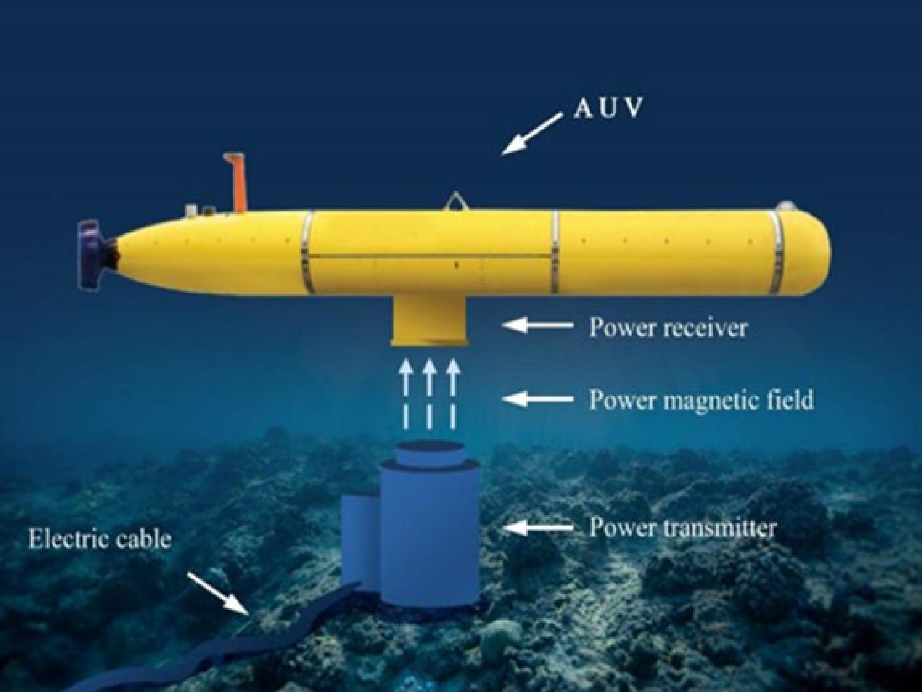
Figure 1.
Schematic of AUV wireless power transfer.
-
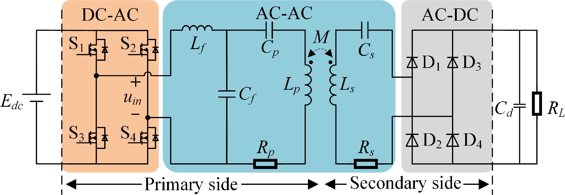
Figure 2.
The WPT system with LCC-S compensation network.
-
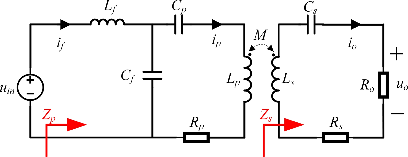
Figure 3.
The equivalent circuit of the system.
-
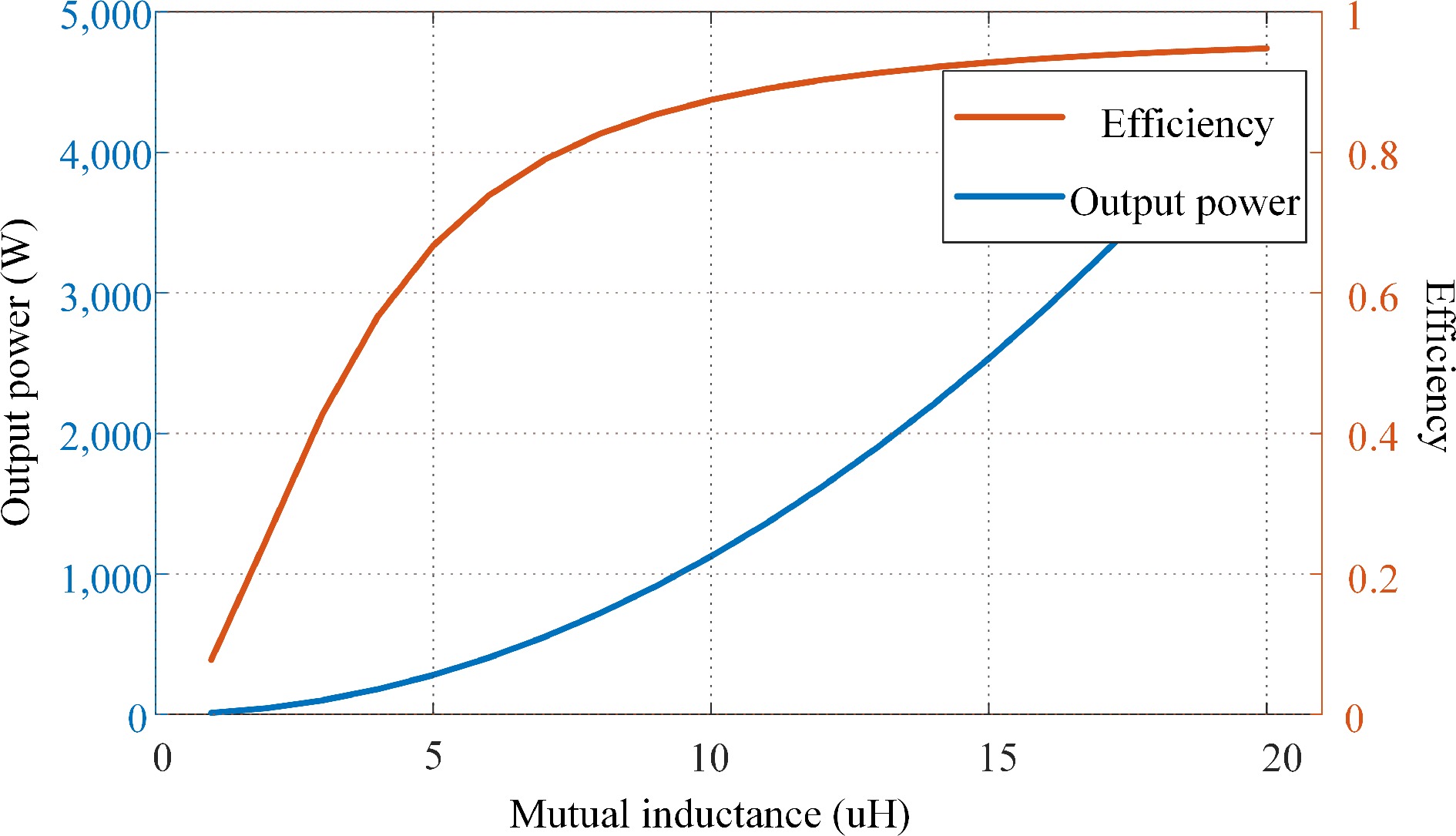
Figure 4.
Output power and efficiency.
-
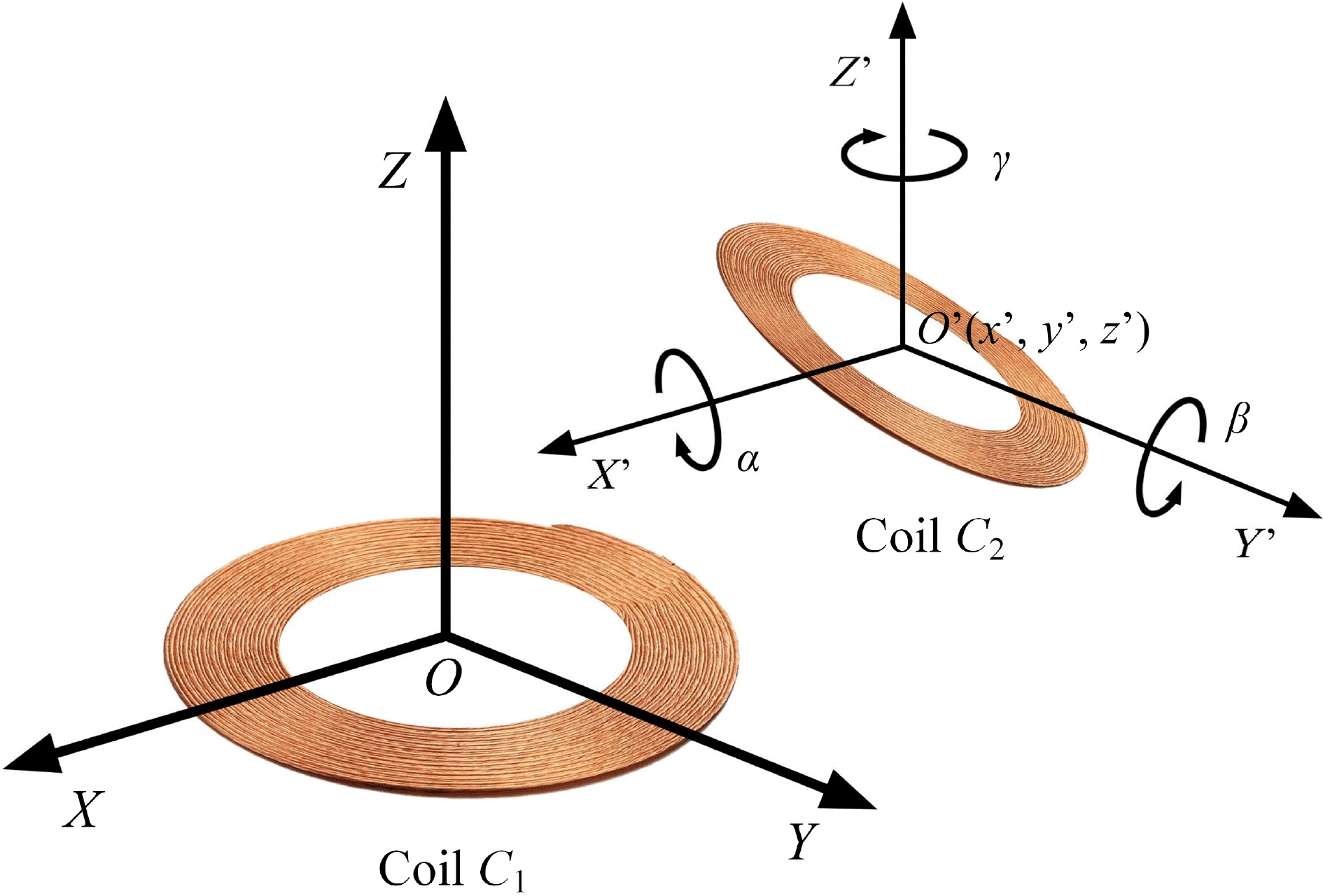
Figure 5.
Positional relation of AUV WPT system coupling mechanism.
-
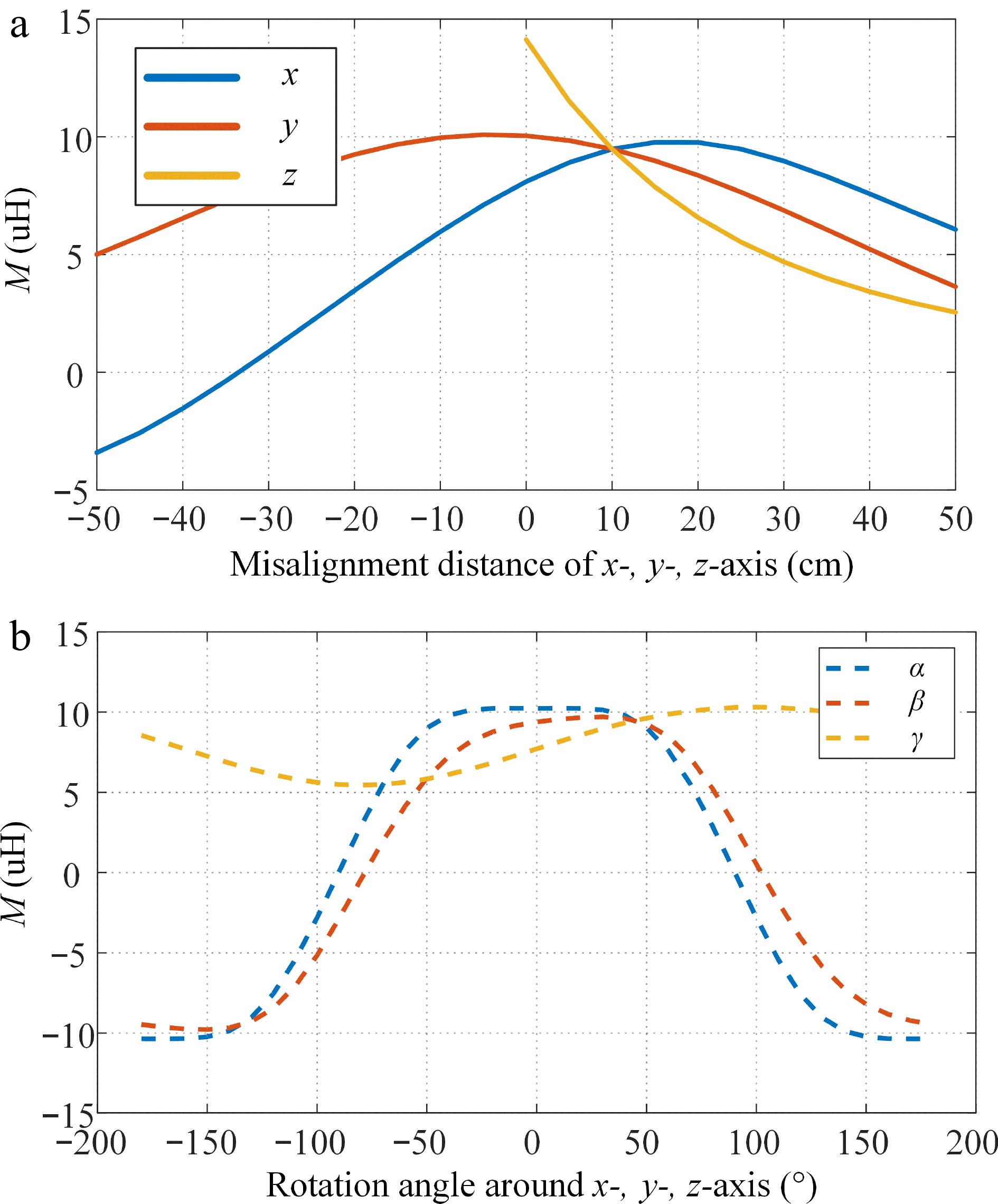
Figure 6.
Mutual inductance M vs (a) misalignment distance, (b) rotational angle.
-
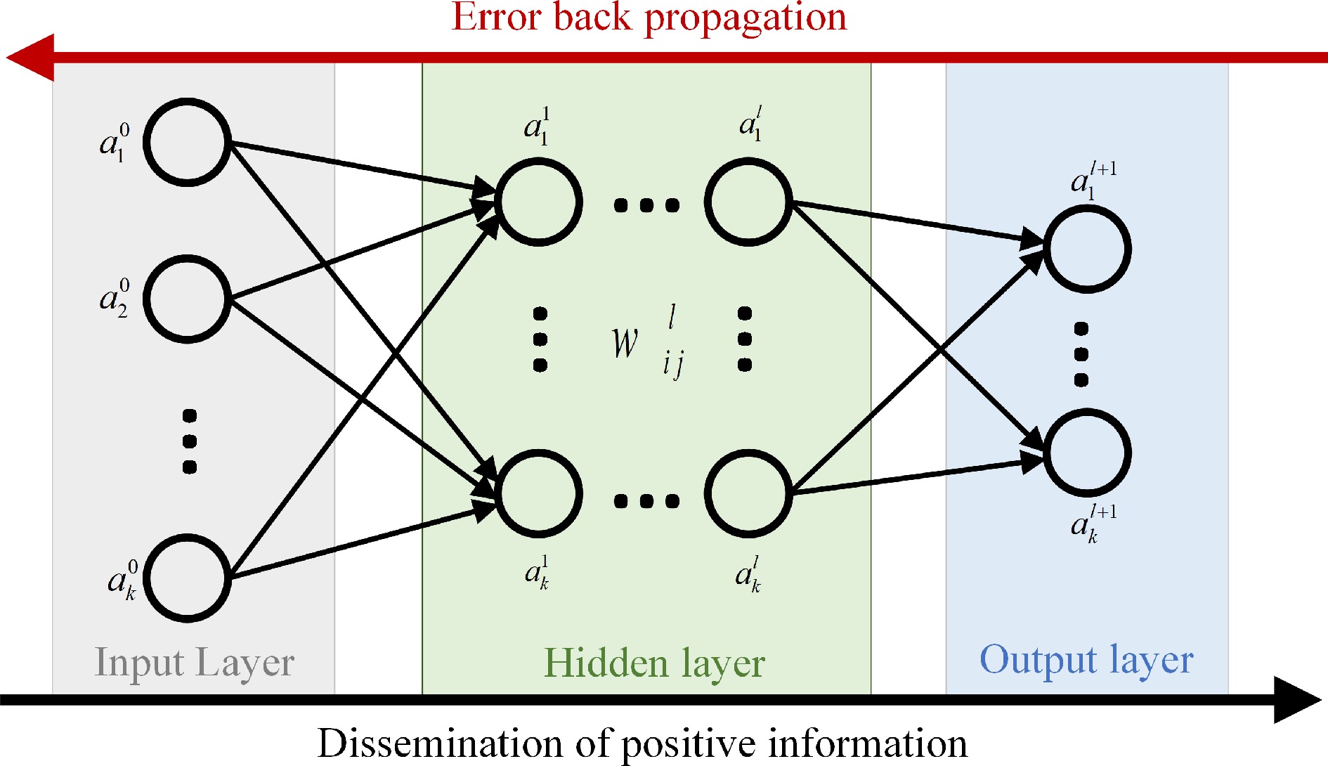
Figure 7.
Neural network architecture.
-
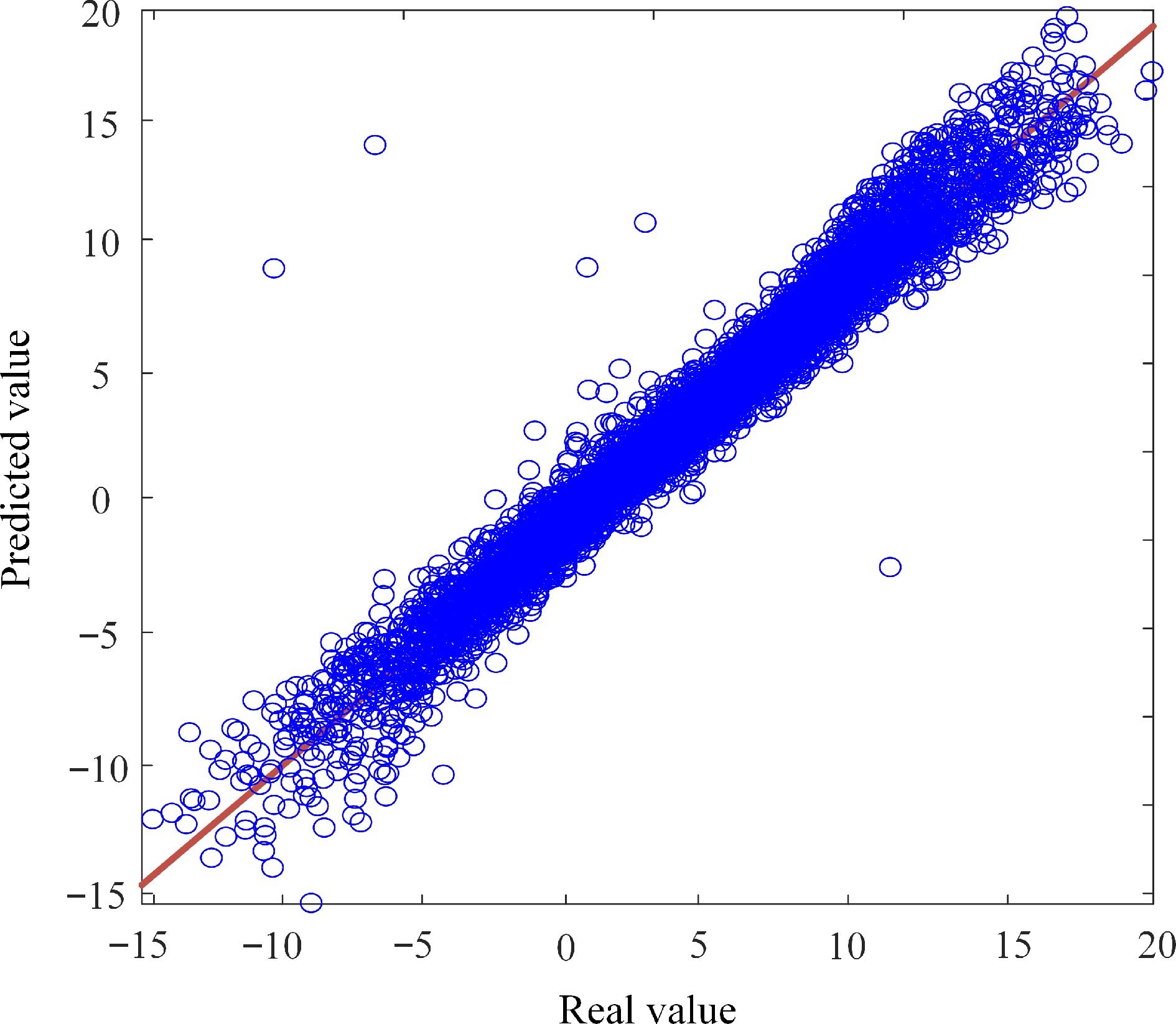
Figure 8.
Comparison between predicted and real mutual inductance values in the testing dataset.
-
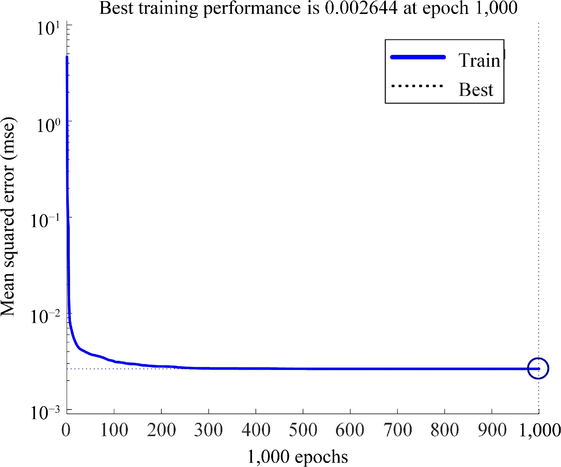
Figure 9.
Convergence process of the surrogate model.
-
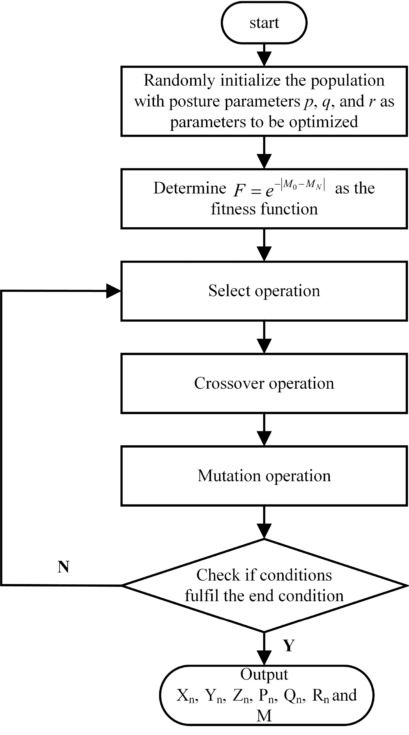
Figure 10.
Genetic algorithm optimization flow chart.
-
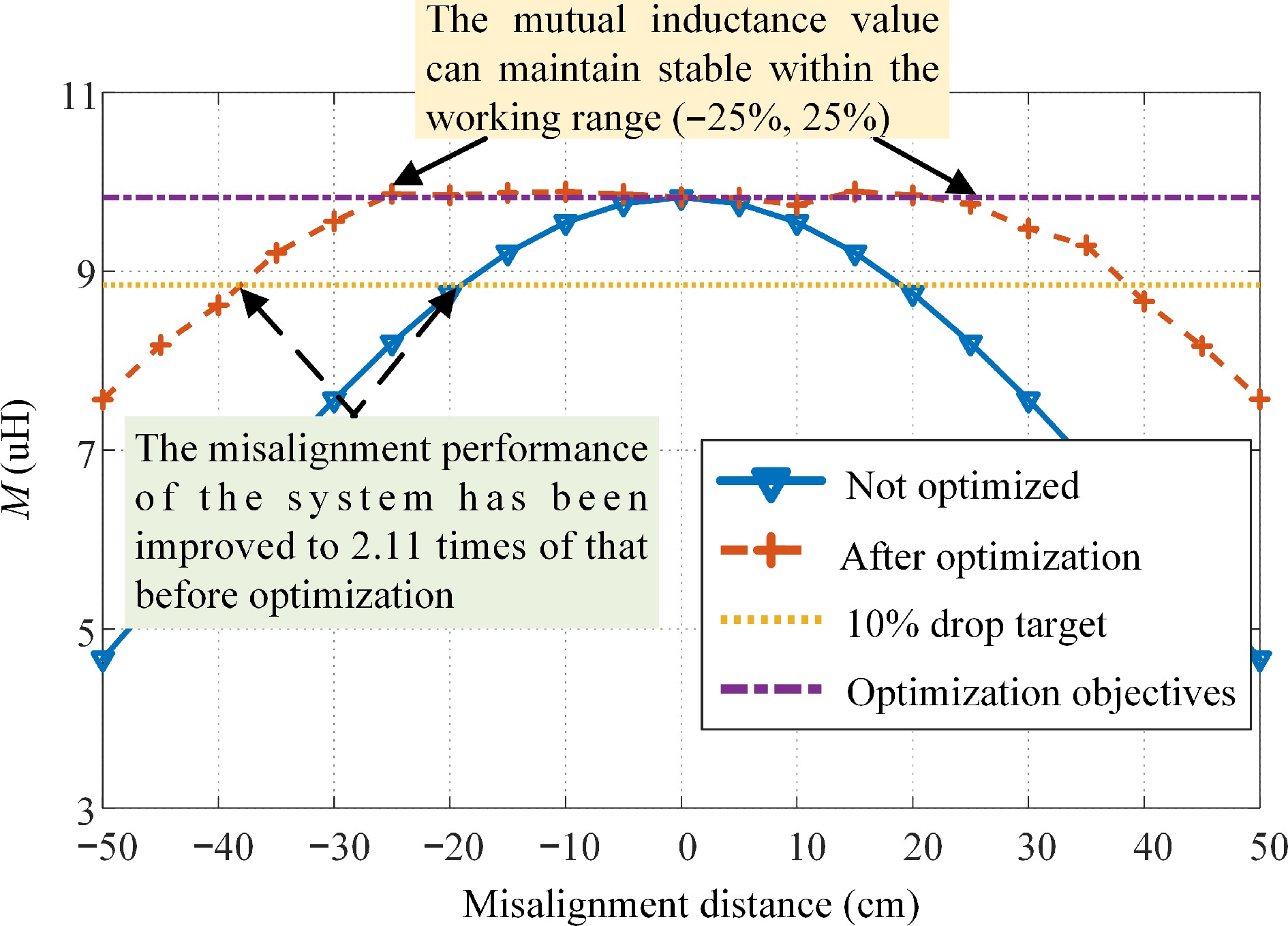
Figure 11.
Comparison of the mutual inductance of the system before and after optimization.
-
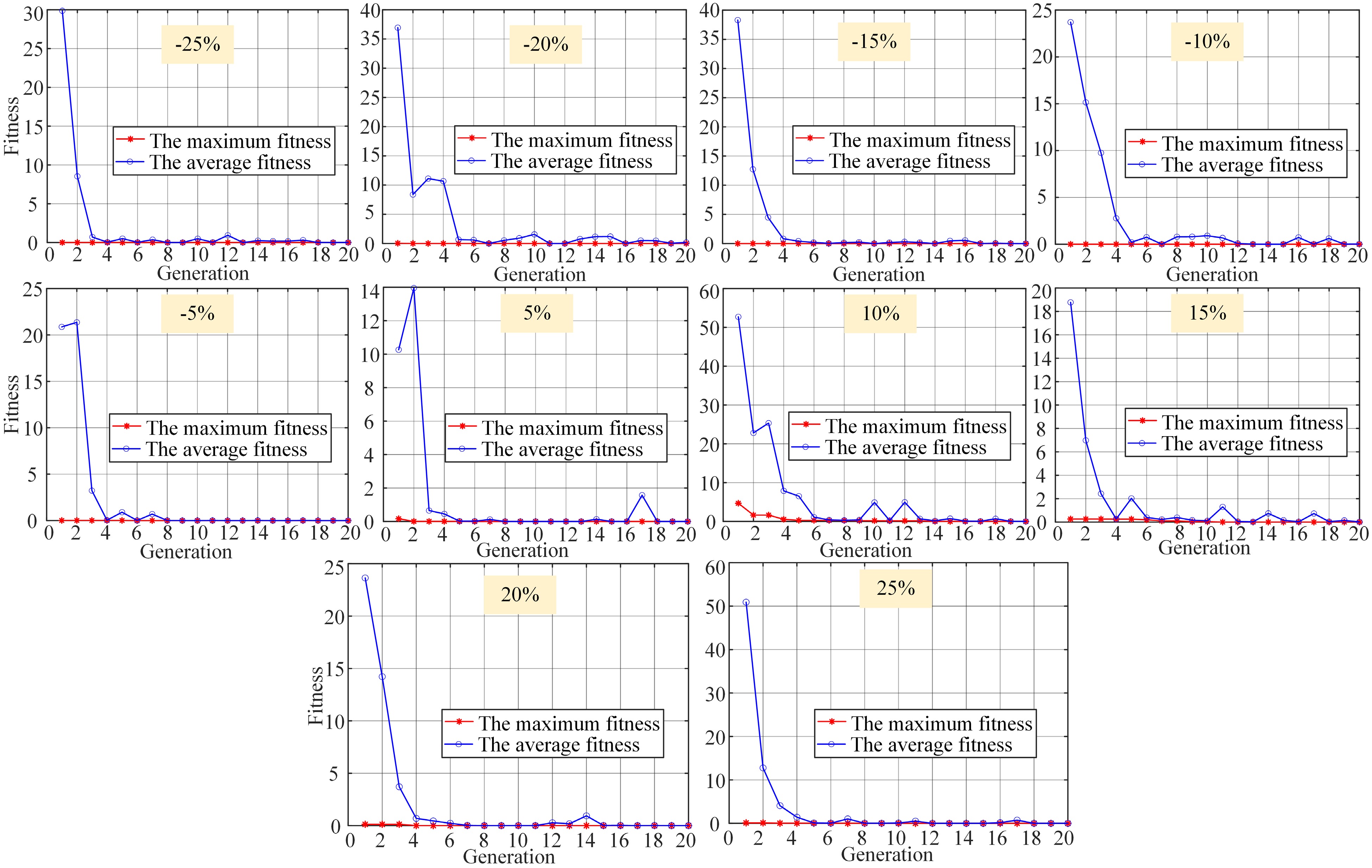
Figure 12.
Test set global optimization convergence process.
-
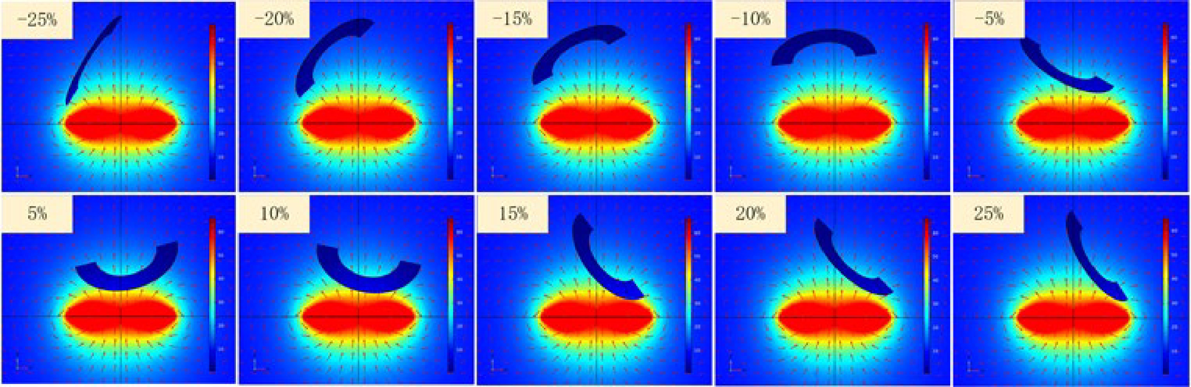
Figure 13.
Electromagnetic field simulation for each test point within the working range.
-
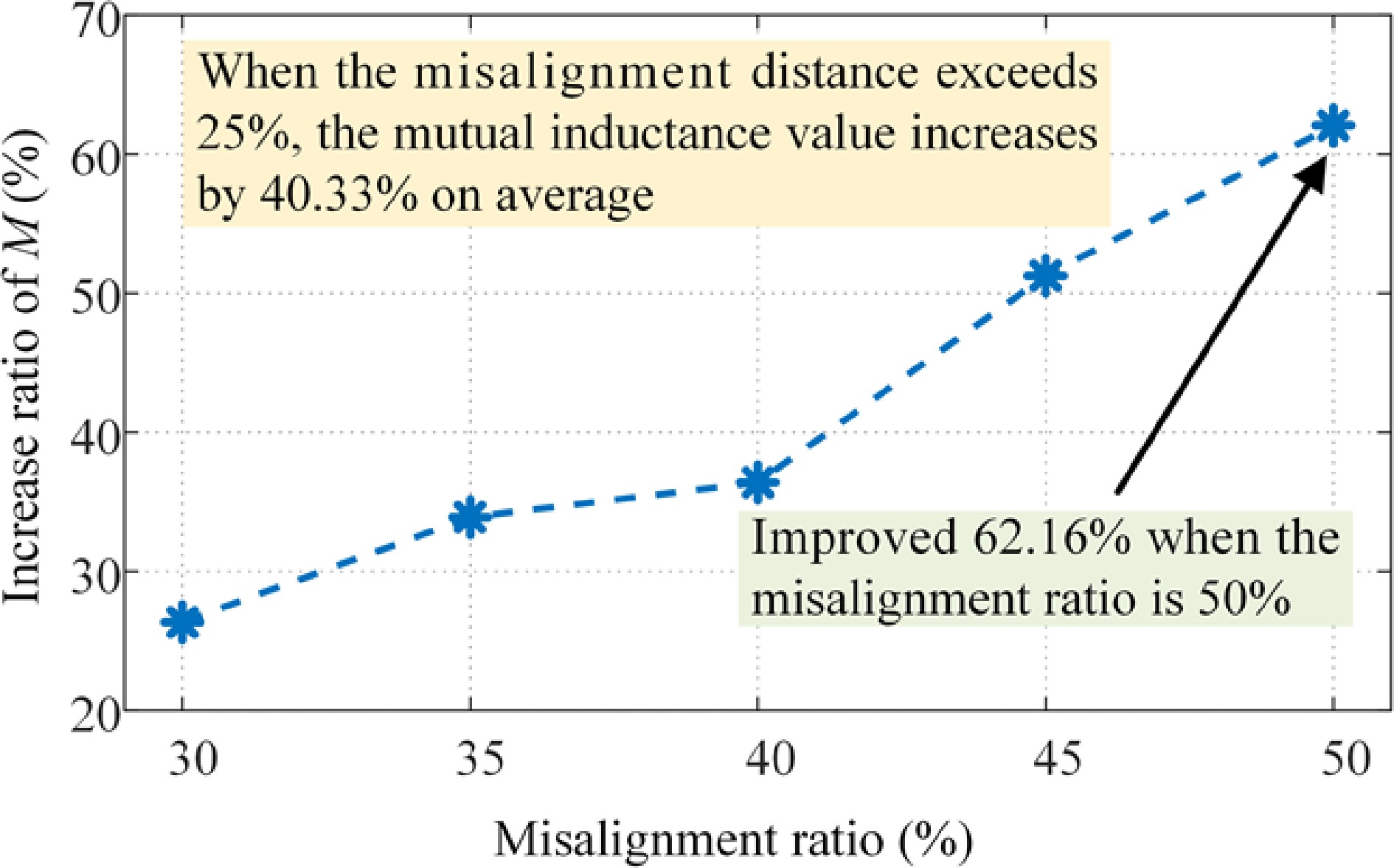
Figure 14.
Improvement of mutual inductance outside of the stable range by the optimization algorithm.
-
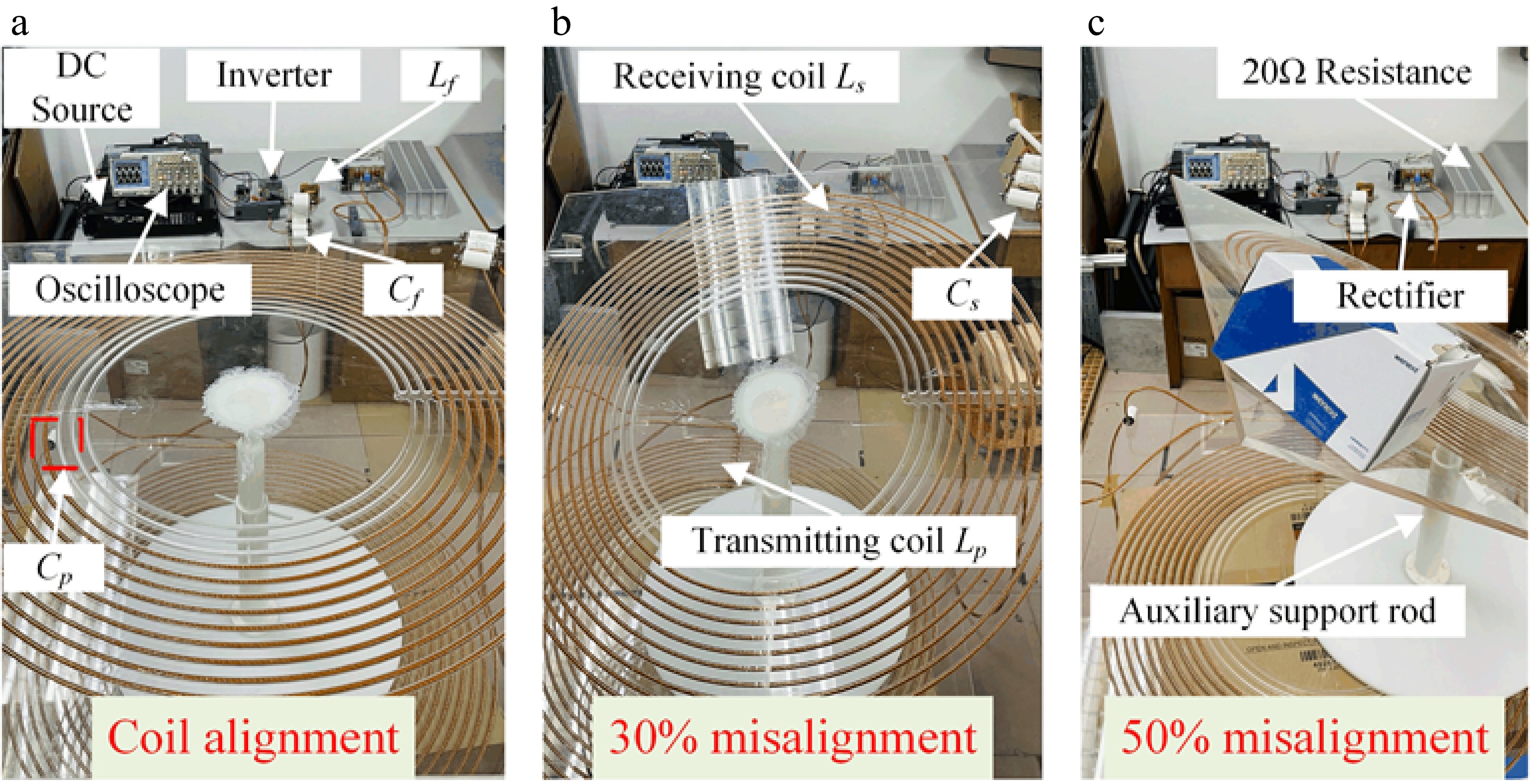
Figure 15.
Experimental prototype. (a) Coil alignment. (b) 30% misalignment. (c) 50% misalignment.
-
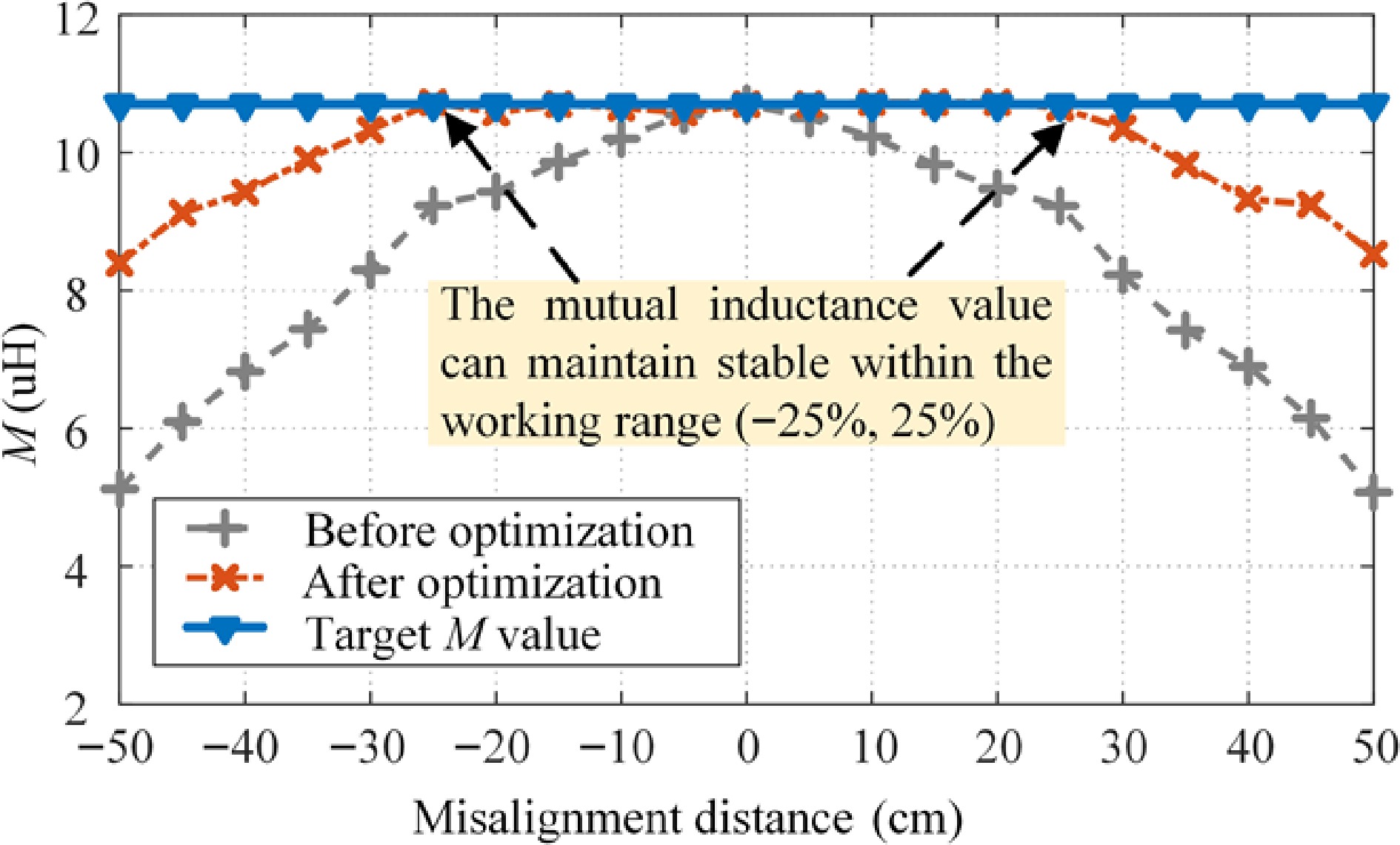
Figure 16.
Comparison curve for mutual inductance M.
-
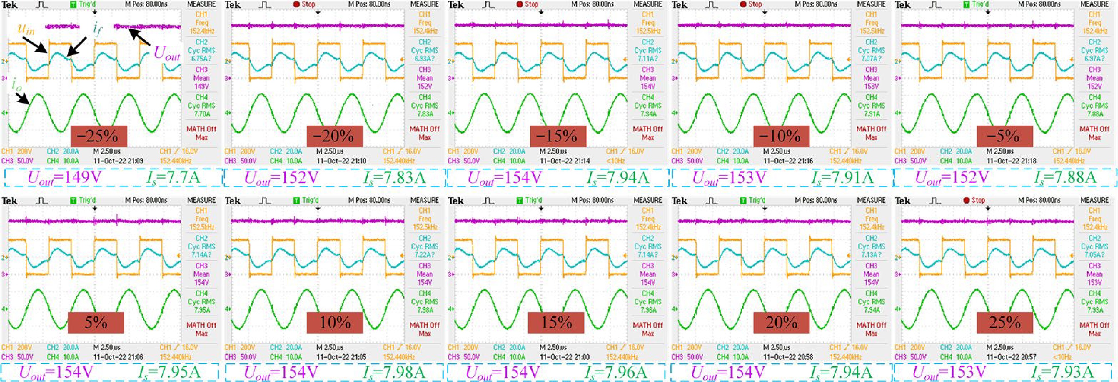
Figure 17.
Experimental waveforms for different misalignment cases with the proposed algorithm adopted.
-
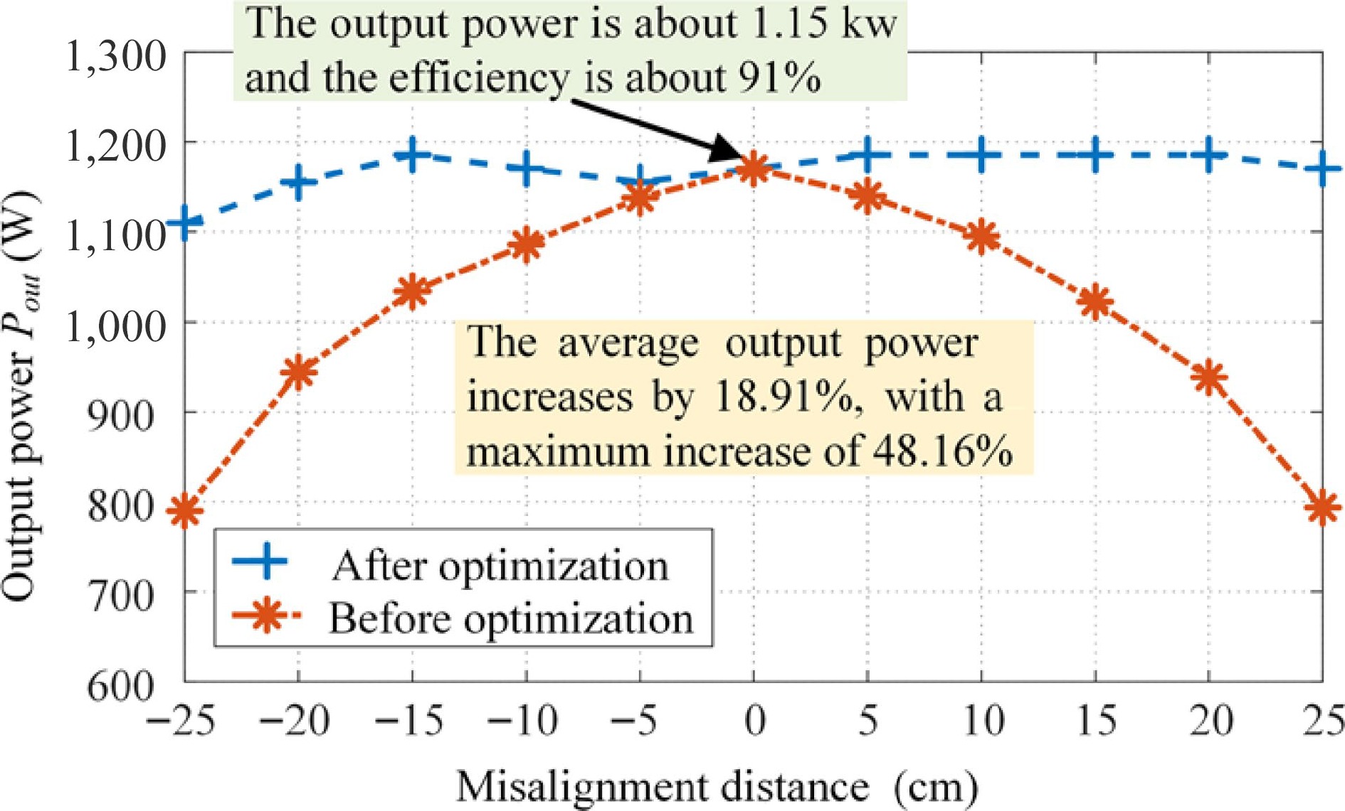
Figure 18.
Comparison curve for output power Pout.
-
Symbol Parameter Value Uin Input voltage 200 V f Frequency 150 kHz Lf Primary compensation inductor 13 µH Cf Primary compensation capacitor 86.6 nF Cp Primary resonance capacitor 10.46 nF Lp Primary side coil 120.6 µH Ls Secondary side coil 121.2 µH Cs Secondary resonance capacitor 9.29 nF Rp Parasitic resistance of Lp 0.48 Ω Rs Parasitic resistance of Ls 0.51 Ω Ro Resistance 20 Ω Table 1.
Coupler parameters.
-
Design parameters Outer diameter Inner diameter No. of turns No. of layers Wire diameter Primary coil 100 cm 60 cm 10 1 3.9 mm Secondary coil 100 cm 60 cm 10 1 3.9 mm Table 2.
Design parameters for coupling mechanisms in AUV UWPT systems.
-
Coupling parameters x (cm) y (cm) z (cm) α (°) β (°) γ (°) Data range [−50.00, 50.00] [−50.00, 50.00] [50.00, 100.00] [−90°, 90°] [−90°, 90°] [−90°, 90°] Table 3.
Range of variation in coupling parameters of AUV UWPT systems.
-
Hyperparameter Search range Number of hidden layers 2, 3, 4 Number of neurons in the hidden layer 16, 32, 64, 128 Batch size 4, 8, 16, 32 Table 4.
Search ranges of hyperparameters.
-
HLN NN BS R2 HLN NN BS R2 HLN NN BS R2 2 16 4 0.9552 3 16 4 0.9396 4 16 4 0.9665 2 16 8 0.8887 3 16 8 0.9584 4 16 8 0.9191 2 16 16 0.9519 3 16 16 0.9484 4 16 16 0.9247 2 16 32 0.9354 3 16 32 0.9492 4 16 32 0.9471 2 32 4 0.9693 3 32 4 0.9450 4 32 4 0.9395 2 32 8 0.9429 3 32 8 0.9621 4 32 8 0.9227 2 32 16 0.9256 3 32 16 0.8998 4 32 16 0.7922 2 32 32 0.9606 3 32 32 0.9060 4 32 32 0.8342 2 64 4 0.9372 3 64 4 0.9580 4 64 4 0.9365 2 64 8 0.9373 3 64 8 0.9645 4 64 8 0.9394 2 64 16 0.8674 3 64 16 0.8492 4 64 16 0.8663 2 64 32 0.9180 3 64 32 0.7726 4 64 32 0.7899 2 128 4 0.9581 3 128 4 0.9444 4 128 4 0.8855 2 128 8 0.8882 3 128 8 0.9446 4 128 8 0.9105 2 128 16 0.8045 3 128 16 0.9018 4 128 16 0.9630 2 128 32 0.8411 3 128 32 0.9550 4 128 32 0.9328 Table 5.
R2 values of surrogate models of different hyperparameter groups.
-
Regression algorithms R2 Polynomial regression 0.76 Support vector machine regression 0.65 K nearest neighbor regression 0.58 Random forest 0.74 BP neural network 0.93 Table 6.
Comparison of accuracies of common regression algorithms for model building.
-
Misalignment distance (cm) Rotation angle p (around x-axis) Rotation angle q (around y-axis) Rotation angle r (around z-axis) Mutual inductance without optimization algorithm (µH) Mutual inductance with optimization algorithm (µH) Optimized target of mutual inductance (µH) Error (µH) –50 86.44 –84.27 –85.64 4.6686 7.5662 9.8265 2.2603 –45 –89.42 49.9 89.83 5.4052 8.1761 9.8265 1.6504 –40 60.22 –59.56 –56.96 6.1473 8.6204 9.8265 1.2061 –35 73.18 45.05 –89.47 6.8746 9.2045 9.8265 0.622 –30 60.15 –35.85 –85.09 7.5657 9.5580 9.8265 0.2685 –25 33.10 –52.27 –51.11 8.1992 9.8658 9.8265 –0.0393 –20 –39.71 –36.58 16.72 8.7536 9.8517 9.8265 –0.0252 –15 –27.41 –31.49 –5.61 9.2086 9.8773 9.8265 –0.0508 –10 –33.45 –11.05 –6.70 9.5472 9.8895 9.8265 –0.063 –5 24.69 30.02 –1.25 9.7558 9.8636 9.8265 –0.0371 0 0 0 0 9.8265 9.8265 9.8265 0 5 17.83 –42.31 49.78 9.7559 9.8213 9.8265 0.0052 10 47.24 –10.61 20.01 9.5472 9.7403 9.8265 0.0862 15 –8.23 59.41 –49.73 9.2086 9.8909 9.8265 –0.0644 20 0.65 50.41 –34.48 8.7534 9.8502 9.8265 –0.0237 25 –3.67 60.82 –31.31 8.1994 9.7524 9.8265 0.0741 30 –58.25 35.81 –87.47 7.5658 9.4767 9.8265 0.3498 35 77.82 29.26 84.01 6.8745 9.2901 9.8265 0.5364 40 85.82 48.16 88.63 6.147 8.6633 9.8265 1.1632 45 89.99 41.02 89.99 5.4055 8.1647 9.8265 1.6618 50 89.99 48.85 89.99 4.6687 7.5706 9.8265 2.2559 Table 7.
Optimization results for each test point and error from the original data.
Figures
(18)
Tables
(7)