


-
Wireless power transfer (WPT) technology has been successfully applied to consumer electronics, mobile devices, electric vehicles (EVs), and many other equipment[1−5]. With the development of marine resources and the marine economy, the scope of autonomous underwater vehicle (AUV) applications has become increasingly wide. Currently, many different types of AUVs are used in various fields, including military applications, petroleum exploration, and scientific research. The battery life is still a challenge, which can be solved using WPT technology.
Given the continuous expansion in the scope of AUV tasks, the use of conventional power supply methods has limited the scope of work and continuous working duration of such vehicles, making power supply the critical factor that determines AUV performance[6−8]. Using emerging, underwater wireless power transfer (UWPT) technology shown in Fig. 1, power can be transmitted without physical contact, enabling galvanic isolation and the elimination of mechanical wear to achieve high reliability, convenience, and safety in an underwater environment[9−11]. Underwater wireless power transfer technology provides a safe and reliable transfer method for AUV underwater power, avoiding the safety hazards caused by underwater wet plugging-unplugging, which has made UWPT a focus of research in the field of wireless power transfer[12−16].
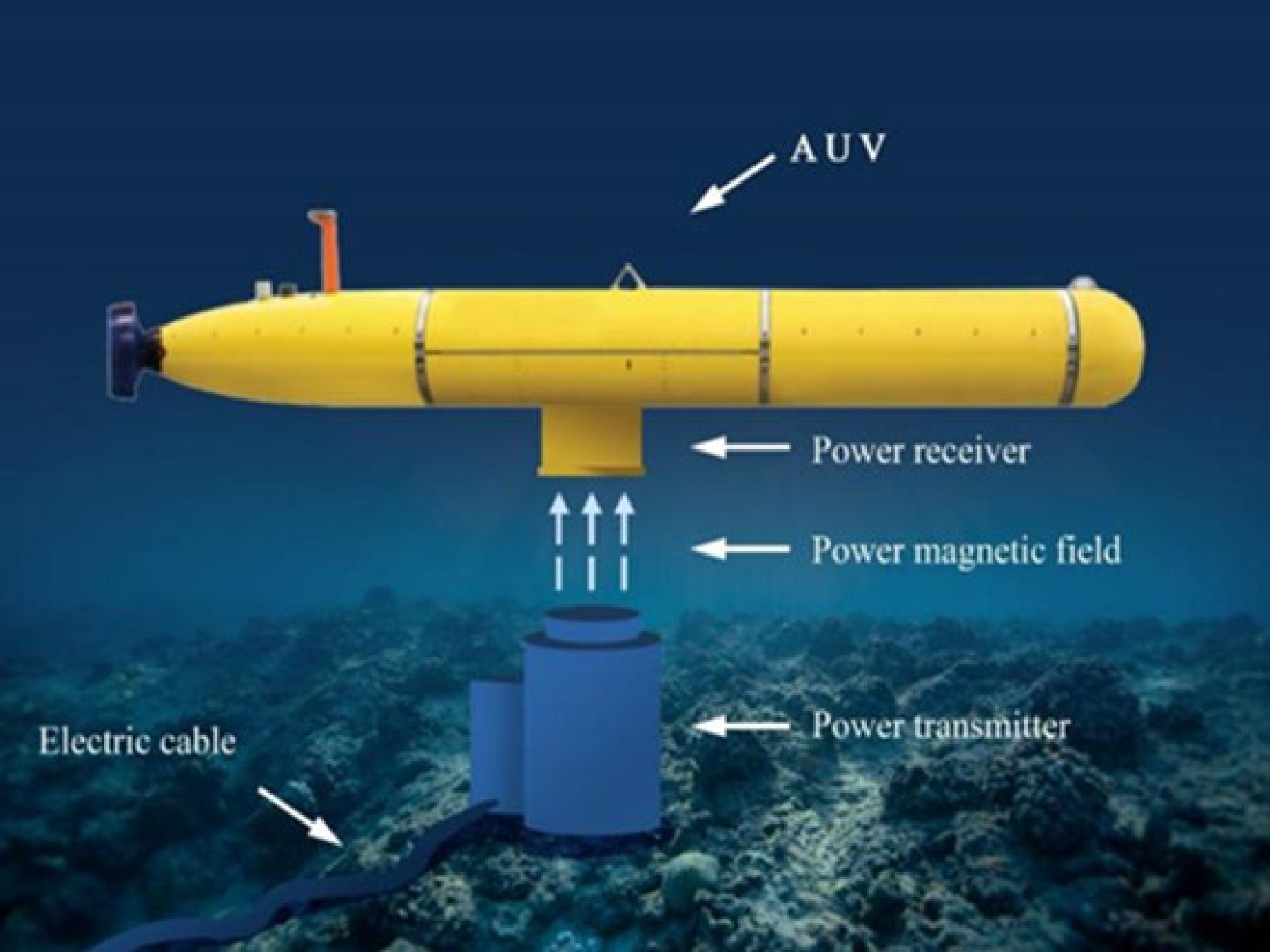
Figure 1.
Schematic of AUV wireless power transfer.
The underwater wireless power transfer environment is influenced by factors that are not found in the atmospheric environment in terms of medium density and ocean currents. In such an environment, misalignments in the coupling mechanism can be more severe and incur greater drops in mutual inductance[17]. The mutual inductance of the coupling mechanism is closely intertwined with the output power, transfer efficiency, and other system indicators[18−24], making it necessary to introduce an anti-misalignment design to ensure the stable operation of the UWPT system. Currently, anti-misalignment problems in the wireless power supplies of AUV are generally resolved using irregular coupling mechanisms such as cage, curly coil, and self-latching coupling mechanisms to attain constant mutual inductance in the coupling mechanism and ensure transfer stability. However, such solutions continue to suffer from drawbacks. The output power of the cage coupling mechanism[25,26] is linked to the relative angle of the coupling mechanism, with a 36.91% difference in the output power between the best and worst cases. The curly coil coupling mechanism[17,27] requires an additional auxiliary mechanism to fix the posture during the charging process, and self-latching coupling mechanisms[28,29] require very high docking precision, making it difficult for AUVs to achieve autonomous self-latching action underwater. Overall, the existing anti-misalignment designs used in UWPT systems sacrifice system flexibility and service life. Simultaneously, problems such as docking difficulties and structural complexities make it crucial to design a power stabilization method with a high degree of freedom.
A free-positioning omnidirectional WPT system with reticulated planar transmitters has been reported[30]. It can use a designed excitation current to generate a three-dimensional (3D) rotating magnetic field to power a receiver at any position and direction. However, as reticulated planar transmitters are large and have low transfer efficiencies (only 55.6%), it is difficult to use them in UWPT systems. New hybrid inductor-capacitor-inductor and capacitor-inductor topologies have also been proposed to resolve the power drop problems caused by the misalignment of wireless charging system coupling mechanisms in electric vehicles[31,32]. The approach utilizes the differing characteristics of the respective topologies under changes in mutual inductance to achieve constant power transfer in a system at a misaligned position; using the optimization algorithm proposed in this paper, the anti-misalignment performance of UWPT systems that apply such topologies can be further improved.
This paper proposes an optimal misalignment posture prediction algorithm for coupling mechanisms based on the mutual inductance surrogate model. The proposed algorithm can attain optimal posture prediction with constant power at any position within the working range. The constant transfer of power in the misaligned state is achieved by adjusting the operating posture of the coupling mechanism. To develop the proposed method, we first established a system circuit theory model for which the mutual inductance of the system was determined as the optimization target. A back propagation (BP) neural network was then used to develop the mutual inductance surrogate model, and the optimal posture with constant power in the misaligned state was finally derived by combining the surrogate model with a genetic algorithm. The contributions of this paper are as follows:
1) An anti-misalignment method for UWPT systems based on a mutual inductance surrogate model and an optimization algorithm is proposed. The mutual inductance surrogate model developed in this study can accurately predict the mutual inductance at any position and posture of a coupling mechanism within its operating range;
2) The surrogate model and genetic algorithm were used to optimize the posture of the coupling mechanism at the misaligned position, thereby achieving constant power transfer in the system in 3D space.
-
To determine the inputs and outputs of the mutual inductance surrogate model, this section focuses on the wireless power transfer system of an AUV with inductance and double capacitances-series (LCC-S) topology and establishes a spatial coordinate system with the geometric center of the primary coil as the origin to determine the relative position and posture parameters of its coupler. Furthermore, an in-depth analysis of the relation between mutual inductance and power transfer characteristics in the LCC-S topology are conducted. The coordinates (x, y, z) of the geometric center of the secondary coil and the rotation angles (α, β, γ) of the secondary coil around the X-, Y-, and Z-axes, respectively, are determined as the inputs of the surrogate model, with mutual inductance output determined as the output. The results provide a theoretical basis for establishing the mutual inductance surrogate model in the next section.
Relation between mutual inductance and system transfer characteristics
-
The LCC-S topology of an AUV wireless power transfer system is modeled and analyzed here and used to develop an equivalent circuit model. The expressions of mutual inductance and the system transfer characteristics are derived from the impedance analysis. The LCC-S circuit diagram is shown in Fig. 2. The primary side of the system in the figure comprises a DC power supply, Edc, high-frequency full bridge inverters (S1–S4), and an LCC network; the secondary side of the system comprises an S network, rectifier, filter capacitor, and load resistor.
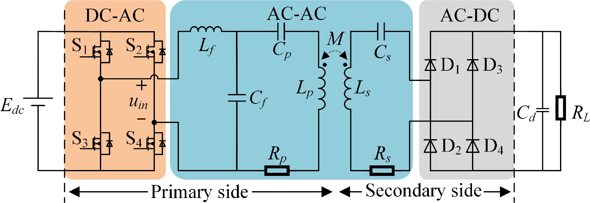
Figure 2.
The WPT system with LCC-S compensation network.
According to the theory of fundamental harmonic approximation, a DC power supply outputs a square wave through an inverter. The power supply and equivalent circuit of the inverter is represented as an AC power supply, UI, in which Ro is the AC equivalent resistance. An equivalent circuit of this system is shown in Fig. 3, in which uin and if represent the output voltage and output current, respectively, of the inverter and ip indicates the current of the primary coil. The self-inductances of the primary and secondary coils of the system are LP and LS, respectively, and their internal resistances are RP and RS, respectively. Lf represents the compensation inductance at the transmitting end of the system, CP and CS represent the compensation capacitors in series with the primary and secondary coils of the system, respectively, Cf indicates the compensation capacitor in parallel at the transmitting end of the system, M represents the mutual inductance between the primary and secondary coils, uo and io represent the input AC voltage and current of the load, respectively.
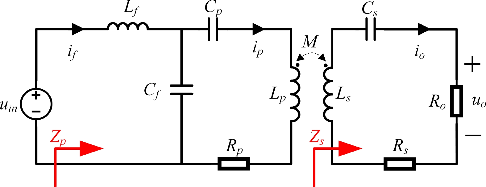
Figure 3.
The equivalent circuit of the system.
The resonance relation of the system is as follows:
$ \left\{ \begin{gathered} j\omega {L_S} + \dfrac{1}{{j\omega {C_S}}} = 0 \\ j\omega {L_f} + \dfrac{1}{{j\omega {C_f}}} = 0 \\ j\omega ({L_P} - {L_f}) + \dfrac{1}{{j\omega {C_P}}} = 0 \\ \end{gathered} \right. $ (1) The impedance ZS of the secondary side can be written as:
$ {Z_S} = {R_S} + {R_O} $ (2) The equivalent load RO is given by:
$ {R_O} = \dfrac{8}{{{\pi ^2}}}{R_L} $ (3) The impedance Zr reflected from the secondary side to the primary side can be expressed as:
$ {Z_r} = \dfrac{{{{(\omega M)}^2}}}{{{R_S} + {R_O}}} $ (4) From this, the impedance Zp of the primary side is:
$ {Z_P} = \dfrac{{{\omega ^2}L_f^2{C_P}({R_O} + {R_S})}}{{\omega {C_P}\left[ {{\omega ^2}{M^2} - j\omega ({L_f} - {L_P})({R_O} + {R_S}) + {R_P}({R_O} + {R_S})} \right] - j{R_O} - j{R_S}}} $ (5) From Eqns (1) to (5), the resonant current If of the primary side of the system, coil current Ip of the primary side, and resonant current IO of the secondary side can be derived as follows:
$ \left\{\begin{array}{l}\dot{{I}_{f}}=\dfrac{\omega {C}_{P}\left[{\omega }^{2}{M}^{2}-j\omega ({L}_{f}-{L}_{P}+{R}_{P})({R}_{O}+{R}_{S})\right]-j({R}_{O}+{R}_{S})}{{\omega }^{2}{L}_{f}^{2}{C}_{P}({R}_{O}+{R}_{S})}\dot{{U}_{I}}\\ \dot{{I}_{P}}=\dfrac{1/j\omega {C}_{f}}{j\omega {L}_{P}+{R}_{P}+{(\omega M)}^{2}/({R}_{S}+{R}_{O})+1/j\omega {C}_{P}+1/j\omega {C}_{f}}\dot{{I}_{I}}\\ \dot{{I}_{O}}=\dfrac{j\omega M}{{R}_{S}+{R}_{O}}\dot{{I}_{P}}\end{array}\right. $ (6) From this, the input and output power of the system are:
$ \left\{\begin{array}{l}{P}_{I}=|\dot{{I}_{f}}{|}^{2}{Z}_{in}=\dfrac{{U}_{I}^{2}({\omega }^{2}{M}^{2}+{R}_{S}{R}_{O}+{R}_{S}{R}_{P})({R}_{O}+{R}_{P})}{2{\omega }^{2}{L}_{f}^{2}{({R}_{O}+{R}_{S})}^{2}}\\ {P}_{O}=|\dot{{I}_{O}}{|}^{2}{R}_{O}=\dfrac{{R}_{O}{U}_{I}^{2}{M}^{2}}{{L}_{f}^{2}{({R}_{O}+{R}_{S})}^{2}}\end{array} \right.$ (7) The efficiency of the system can be simplified as:
$ \eta = \dfrac{{{P_O}}}{{{P_I}}} = \dfrac{{{\omega ^2}{M^2}{R_O}}}{{({\omega ^2}{M^2} + {R_P}{R_O} + {R_S}{R_P})({R_O} + {R_S})}} \times 100{\text{%}} $ (8) Table 1 lists the parameters of the LCC-S topology AUV wireless power transfer system. Figure 4 shows the relation between the power, efficiency, and mutual inductance of the system. From the figure, the output power increases with the mutual inductance and the efficiency of the system increases with the mutual inductance when the inductance is small and then gradually stabilizes. Thus, the mutual inductance of the coupling coil should be increased to its maximum value to increase the output power.
Table 1. Coupler parameters.
Symbol Parameter Value Uin Input voltage 200 V f Frequency 150 kHz Lf Primary compensation inductor 13 µH Cf Primary compensation capacitor 86.6 nF Cp Primary resonance capacitor 10.46 nF Lp Primary side coil 120.6 µH Ls Secondary side coil 121.2 µH Cs Secondary resonance capacitor 9.29 nF Rp Parasitic resistance of Lp 0.48 Ω Rs Parasitic resistance of Ls 0.51 Ω Ro Resistance 20 Ω 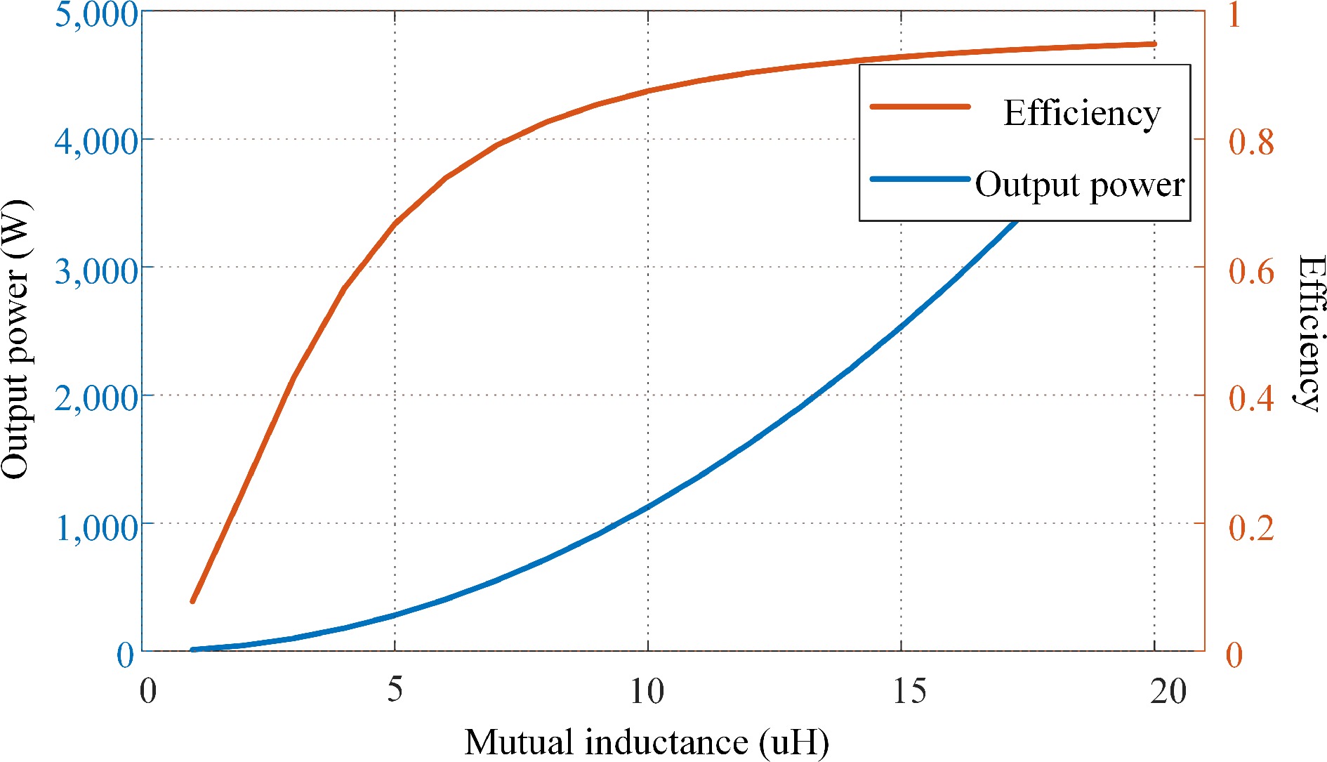
Figure 4.
Output power and efficiency.
The theoretical analysis above indicates that, in an LCC-S topology adopted by an AUV underwater wireless charging system, the mutual inductance is positively correlated with the transfer characteristics of the system under a constant-load scenario. Changes in mutual inductance will cause fluctuations in the transfer characteristics of the system and will have a particularly significant impact on output power.
Relation between the relative position and posture of the coupling mechanism and the mutual inductance
-
In the following analysis, the geometric center of the primary coil is treated as the origin of a spatial Cartesian coordinate system. In the next section, the relative position and posture of the coupling mechanism are parameterized to facilitate the construction of a mutual inductance surrogate model.
Figure 5 shows the positional relations of the coupling mechanism of the AUV wireless power transfer system, with C1 indicating the primary coil fixed at the charging base station and C2 the secondary coil, which is installed on the AUV and can be rotated around its geometric center. Using the Euler angles of a rigid body rotating around a fixed point in a mechanical system[33] and considering all six degrees of freedom describing a spatial position, a 3D coordinate system can be constructed with the geometric center of the primary coil as the origin. In the figure, (x, y, z) represent the coordinates of the geometric center of the secondary coil and (α, β, γ) represent the angles through which the secondary coil rotates around the X-, Y-, and Z-axes, respectively.
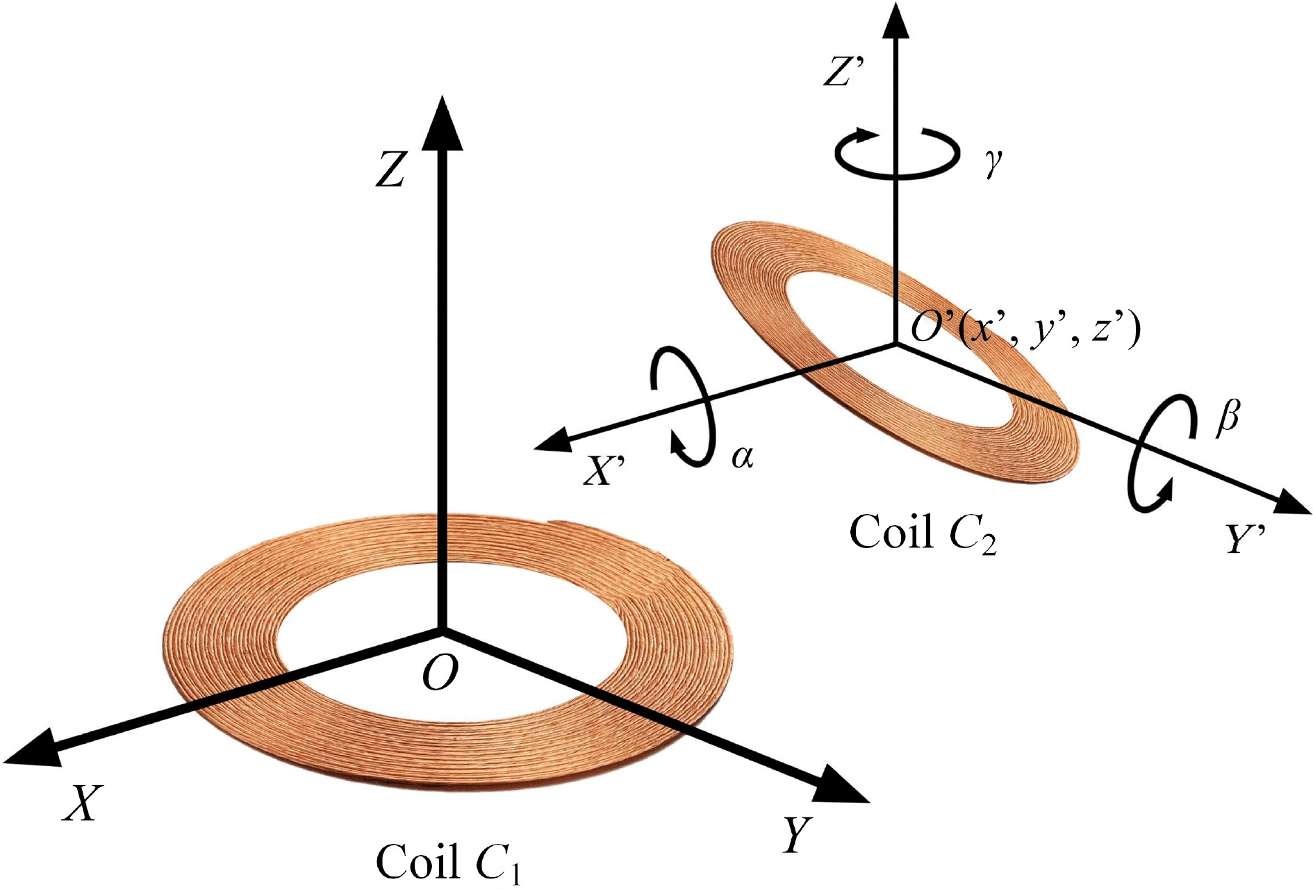
Figure 5.
Positional relation of AUV WPT system coupling mechanism.
According to Neumann’s law, the mutual inductance between primary and secondary coils at any spatial position can be derived as
$ M = \dfrac{{{N_1}{N_2}{u_w}}}{{4\pi }}\oint {\oint {\dfrac{{d\vec{{l_1}} \cdot d\vec {{l_2}} }}{{{r_{12}}}}} } $ (9) where, M represents the mutual inductance between the primary and secondary coils, N1 and N2 indicate the number of turns in the primary and secondary coils, respectively, uw represents the average magnetic permeability in seawater,
$ d\vec {{l_1}} $ $ d\vec {{l_2}} $ $ d\vec {{l_1}}$ $ d\vec {{l_2}} $ The mutual inductance of the primary and secondary coils, which have relatively complex structures with multiple turns, can be established in terms of the parameters of the 3D spatial coordinate system with the origin at the geometric center of the primary coil:
$ M = f(x,y,z,\alpha ,\beta ,\gamma ) $ (10) The relations between independent changes in each parameter and the mutual inductance are shown in Fig. 6. The initial state of rotation is x = 10, y = 10, z = 50, α = 45°, β = 45°, γ = 45°. This analysis reveals that the mutual inductance of an AUV wireless power transfer system is directly related to the relative position and posture of the coupling mechanism, with a change in any one of the selected parameters causing a change in the mutual inductance. However, the manner in which the mutual inductance is altered differs by parameter. In practical applications, adjusting a single parameter is insufficient to meet control requirements, and the system must be optimized globally. To achieve this, we establish a mutual inductance surrogate model in the following section.
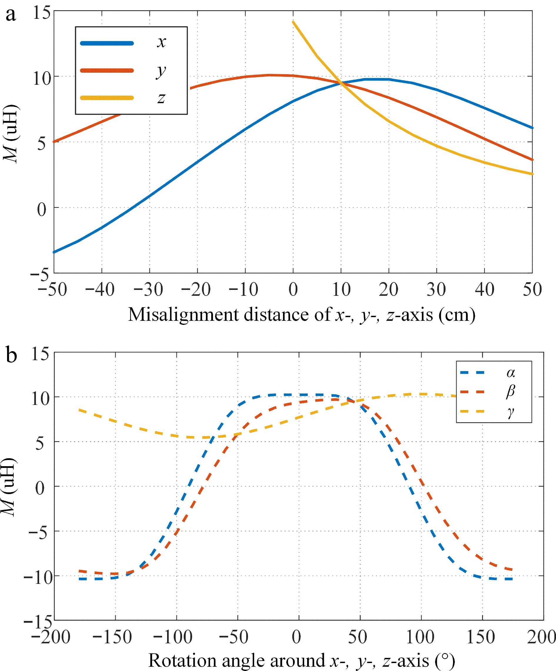
Figure 6.
Mutual inductance M vs (a) misalignment distance, (b) rotational angle.
-
As the measurement of mutual inductance during a dynamic process is very time-consuming, appropriate measuring equipment must be used. The relation between the relative position and posture of the primary and secondary coils and the transfer characteristics of the system is also extremely complicated, and the mutual inductance and transfer characteristics of the AUV wireless charging system LCC-S topology exhibits a positive correlation. To achieve global optimization of the mutual inductance parameters, we used a BP neural network to develop a mutual inductance surrogate model of the AUV wireless power transfer system that can predict the mutual inductance at any relative position and posture of the coupling mechanism. The Latin hypercube sampling method (LHS) was used to construct sample points for which the mutual inductance values were numerically simulated using the COMSOL software. Ten-fold cross-validation was used to avoid overfitting the surrogate model. The surrogate model developed in this section provides a model foundation for the posture optimization of the secondary coil under constant power transfer, as described in the next section. Other parameters of the coupling mechanism are listed in Table 2.
Table 2. Design parameters for coupling mechanisms in AUV UWPT systems.
Design parameters Outer diameter Inner diameter No. of turns No. of layers Wire diameter Primary coil 100 cm 60 cm 10 1 3.9 mm Secondary coil 100 cm 60 cm 10 1 3.9 mm Numerical simulation and dataset creation
-
The LHS method was used to establish the sample space for the surrogate model. For each sampling point, the relative coordinates x, y, and z between the secondary and primary coils and the angles α, β, and γ of the secondary coil around the coordinate axis were selected as input variables and the mutual inductance of the coupling mechanism was selected as the output variable. LHS is an approximate random sampling method based on a multivariate parameter distribution and constitutes a stratified sampling technique with uniform stratification. LHS is able to construct models more effectively in sample spaces with high latitudes and low sample numbers. The ranges of all coupling parameters were defined based on the actual working area of the coupling coil, as shown in Table 3. A total of 10,000 sample points with different values of x, y, z, α, β, and γ were identified, 7,000 of which were used as the training set to determine the parameters of the surrogate model. The remaining 3,000 sample points were used as a test set to evaluate the predictive performance of the surrogate model. Using COMSOL software, a finite element model of each sample point was established and the electromagnetic field characteristics of the model were calculated, thereby obtaining the mutual inductance of the system.
Table 3. Range of variation in coupling parameters of AUV UWPT systems.
Coupling parameters x (cm) y (cm) z (cm) α (°) β (°) γ (°) Data range [−50.00, 50.00] [−50.00, 50.00] [50.00, 100.00] [−90°, 90°] [−90°, 90°] [−90°, 90°] Construction of mutual inductance surrogate model based on BP neural network
-
A multi-layer forward neural network based on error backpropagation was used to construct the surrogate model. As the activation function of a BP neural network is usually a sigmoid function that is continuously differentiable, any non-linear mapping between the input and output can be attained. Therefore, such networks are most extensively applied in pattern recognition, risk assessment, and adaptive control. The BP neural network design was initially researched and designed by Rumelhart et al.[34].
Figure 7 shows the architecture of a BP neural network. The main structure comprises an input layer, one or more hidden layers, and an output layer. Each layer comprises several neurons, with the output of each neuron determined by its input value, effect function, and threshold value. In the figure,
$a_j^l$ $ w_{ij}^l $ $b_j^l$ $\sigma $ 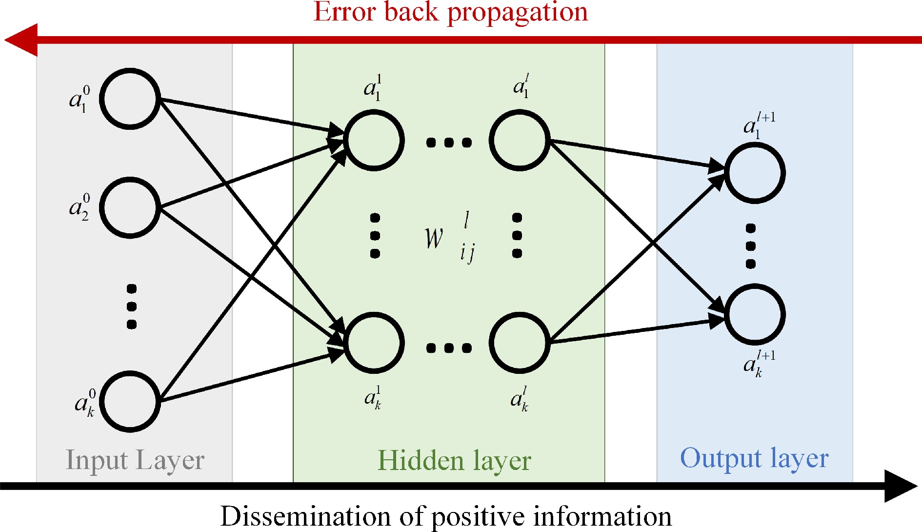
Figure 7.
Neural network architecture.
$ a_j^l = \sigma (\sum\limits_k {{w_{jk}^l}a_k^{l - 1} + b_j^l} ) $ (11) where L and α denote the loss function and learning rate, respectively, of the network. According to the gradient descent principle, the parameter update rule of the mutual inductance surrogate model can be given as:
$ \left\{ \begin{gathered} {b^l} \leftarrow {b^l} - \alpha \dfrac{{\partial L}}{{\partial {b^l}}} \\ {w^l} \leftarrow {w^l} - \alpha \dfrac{{\partial L}}{{\partial {w^l}}} \\ \end{gathered} \right. $ (12) In building a BP neural network, all hyperparameters, including the learning rate, batch size, number of neurons, and number of hidden layers, must be fixed before model training begins. The performance of most machine learning models is largely determined by the choice of hyperparameters, with common hyperparameter optimization approaches used in current optimization methods including grid search, random search, and Bayesian optimization. As the principle of grid search is simple and suitable for cases with few hyperparameters, grid search was used to optimize the hyperparameters of the network.
Based on the theoretical analysis above, the number of neurons in the input and output layers were set as six and one, respectively, with the hyperparameters to be determined including the learning rate, activation function, batch size, number of neurons, and number of hidden layers. The Adam adaptive optimization algorithm[35] can be used to automatically adjust the learning rate. Although there is no approach in the existing literature providing a direct formula for adjusting the batch size, it has been proposed[36] that the optimal batch size lies within a range of 2 to 32. There is also no current theory for determining the optimal number of hidden layers and neurons required by a neural network to solve certain problems. In general, a neural network model with two to three hidden layers will have a sufficiently robust non-linear fitting ability to resolve most problems, and setting the same number of neurons in each hidden layer enables very good neural network model performance. Based on the factors described above, the ranges of values of hyperparameters that needed to be determined via the grid search method are listed in Table 4.
Table 4. Search ranges of hyperparameters.
Hyperparameter Search range Number of hidden layers 2, 3, 4 Number of neurons in the hidden layer 16, 32, 64, 128 Batch size 4, 8, 16, 32 The mean squared error (MSE), mean absolute error (MAE), and coefficient of determination (R2) were used to evaluate the training performance and generalizability of the surrogate model using the following evaluation metrics:
$ MAE = \dfrac{1}{N}\sum\limits_{i = 1}^N {\left| {{y_i} - {{y'_i}}} \right|} $ (13) $ MSE = \dfrac{1}{N}\sum\limits_{i = 1}^N {({y_i} - {{y'_i}}} {)^2} $ (14) $ {R^2} = {{1 - \sum\limits_{i = 1}^N {{{({y_i} - {{y'_i}})}^2}} } \mathord{\left/ {\vphantom {{1 - \sum\limits_{i = 1}^N {{{({y_i} - {{y'_i}})}^2}} } {\sum\limits_{i = 1}^N {{{({y_i} - \bar y)}^2}} }}} \right. } {\sum\limits_{i = 1}^N {{{({y_i} - \bar y)}^2}} }} $ (15) Table 5 lists the relative error of the neural network model that corresponds to each set of hyperparameters in the grid search after the same number of iterations, where HLN represents the number of hidden layers, NN represents the number of neurons in the hidden layer, BS represents the batch size, and R2 represents the coefficient of determination between the predicted value of the model and the actual value. From Table 5, a network with two hidden layers, 32 neurons in each hidden layer, and a batch size of five achieves the best performance, with an R2 of 0.9693.
Table 5. R2 values of surrogate models of different hyperparameter groups.
HLN NN BS R2 HLN NN BS R2 HLN NN BS R2 2 16 4 0.9552 3 16 4 0.9396 4 16 4 0.9665 2 16 8 0.8887 3 16 8 0.9584 4 16 8 0.9191 2 16 16 0.9519 3 16 16 0.9484 4 16 16 0.9247 2 16 32 0.9354 3 16 32 0.9492 4 16 32 0.9471 2 32 4 0.9693 3 32 4 0.9450 4 32 4 0.9395 2 32 8 0.9429 3 32 8 0.9621 4 32 8 0.9227 2 32 16 0.9256 3 32 16 0.8998 4 32 16 0.7922 2 32 32 0.9606 3 32 32 0.9060 4 32 32 0.8342 2 64 4 0.9372 3 64 4 0.9580 4 64 4 0.9365 2 64 8 0.9373 3 64 8 0.9645 4 64 8 0.9394 2 64 16 0.8674 3 64 16 0.8492 4 64 16 0.8663 2 64 32 0.9180 3 64 32 0.7726 4 64 32 0.7899 2 128 4 0.9581 3 128 4 0.9444 4 128 4 0.8855 2 128 8 0.8882 3 128 8 0.9446 4 128 8 0.9105 2 128 16 0.8045 3 128 16 0.9018 4 128 16 0.9630 2 128 32 0.8411 3 128 32 0.9550 4 128 32 0.9328 Training of mutual inductance surrogate model
-
Using the dataset created previously, and the mutual inductance surrogate model established by the BP neural network algorithm, the relative position parameters (x, y, z) and posture parameters (α, β, γ) were set as input variables and the mutual inductance M was set as the output variable. The dataset of 10,000 sample points was divided into two subsets: one with 7,000 sample points to train and validate the surrogate model and another with 3,000 sample points to test the model. To obtain as much effective information as possible from the limited data and prevent overfitting of the surrogate model, a 10-fold cross-validation method was used to construct the surrogate model via the following steps:
1) Divide the subset of 7,000 sample points into 10 groups, with each group including the same number of sample points randomly selected from the subset;
2) Construct 10 models. In the training and validation of each model, one group is selected as the validation dataset and the remaining nine are used as the training dataset. The model is trained using the training datasets and its R2 value is calculated using the validation dataset;
3) The output of the 10 training models is averaged to give the output of the surrogate model.
The R2 values of the 10 models in the validation dataset were 0.9045, 0.9619, 0.9620, 0.9610, 0.9551 0.9531, 0.9636, 0.9247, 0.9642, and 0.9591, respectively. The generalizability of the surrogate model was tested using the 3,000-sample-point test dataset. A comparison between the mutual inductance predicted by the surrogate model and that determined by the numerical simulation of the test dataset is shown in Fig. 8, with the convergence process of the surrogate model shown in Fig. 9. The R2 value of the surrogate model was 0.9328, indicating that the model had robust generalizability. Using the surrogate model with the position parameters of the secondary coil relative to the primary coil in 3D space and posture parameters of the secondary coil as inputs, the mutual inductance of the coupling mechanism can be determined quickly and effectively.
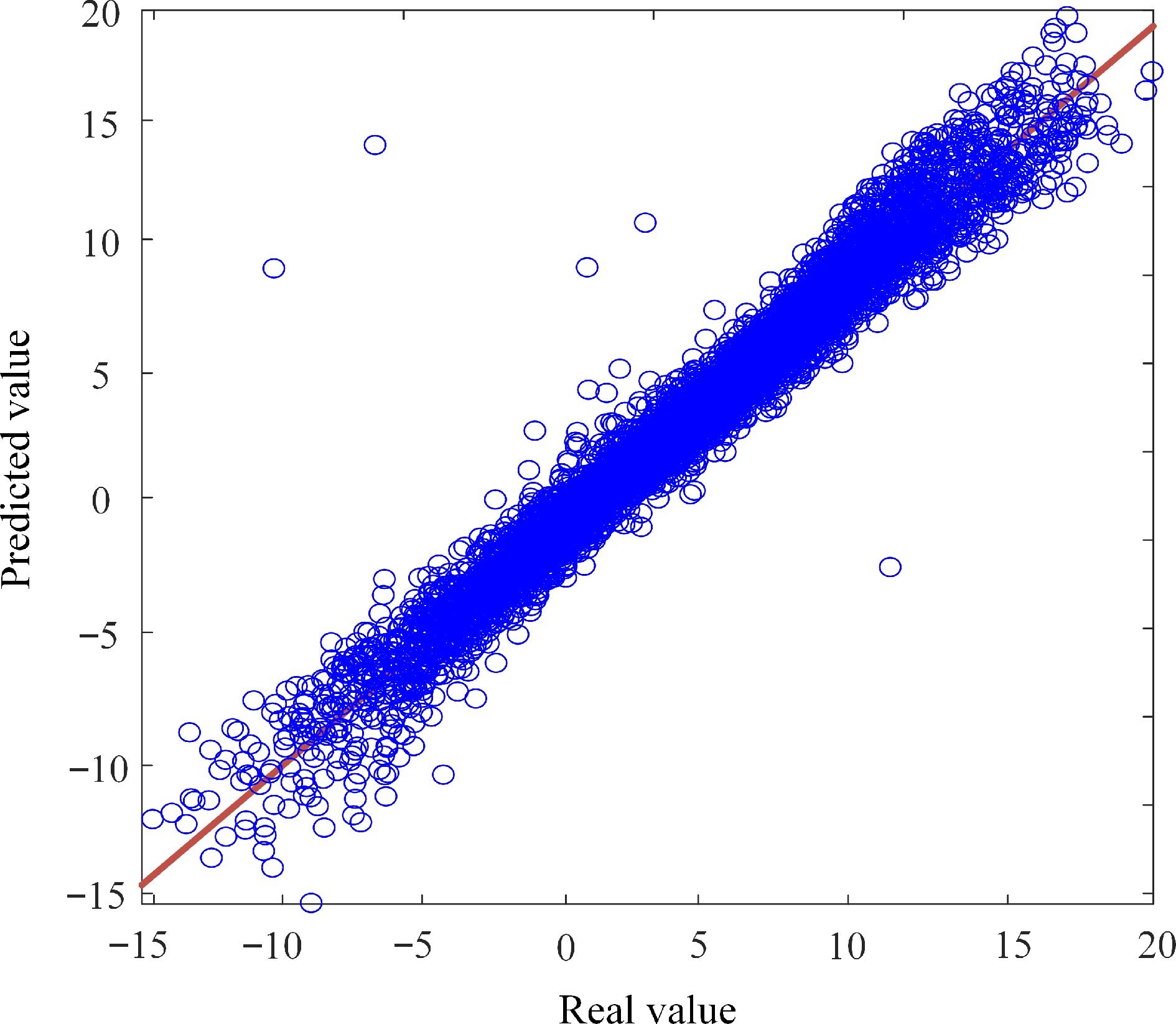
Figure 8.
Comparison between predicted and real mutual inductance values in the testing dataset.
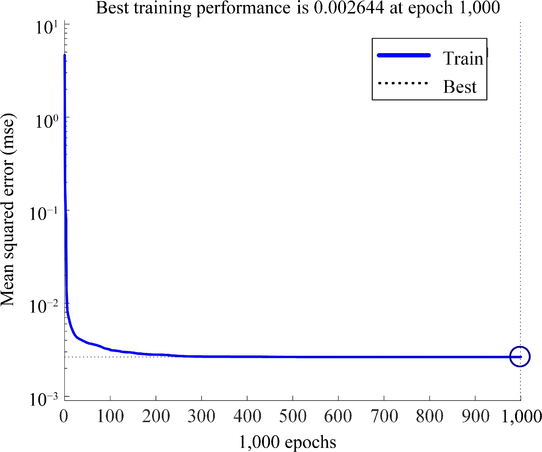
Figure 9.
Convergence process of the surrogate model.
It was important to further verify the selected neural network regression algorithm, in particular in terms of its effectiveness and accuracy, to ensure that the constructed surrogate model provided the best performance in terms of model accuracy. After determining the hyperparameters of the neural network model, its accuracy was compared against those of commonly used regression algorithms for the construction of UWPT mutual inductance surrogate models, as shown in Table 6. It can be observed from the table that the R2 value corresponding to the proposed neural network algorithm is the largest, indicating that its accuracy in constructing system energy efficiency models is significantly better than that of other regression algorithms.
Table 6. Comparison of accuracies of common regression algorithms for model building.
Regression algorithms R2 Polynomial regression 0.76 Support vector machine regression 0.65 K nearest neighbor regression 0.58 Random forest 0.74 BP neural network 0.93 Genetic algorithm for the posture optimization of coupling mechanisms with constant power transfer at misaligned positions
-
The surrogate model developed in the previous section can be used to quickly predict the mutual inductance of an AUV wireless power transfer system under different relative positions and postures. Here, we describe how a genetic algorithm, working with the surrogate model in an iterative process, can be applied in conditions in which the misaligned position is known to optimize the optimal posture of the secondary coil for constant power transfer at the misaligned position.
The genetic algorithm, an evolutionary computing technique proposed by John Holland and based on the law of evolution of organisms in nature, is a method for searching for an optimal solution by simulating natural evolutionary processes. The algorithm mathematically converts the problem-solving process into a process similar to the crossing over and mutation of chromosome genes in biological evolution. It is able to obtain better optimization results than conventional optimization algorithms in solving more complex combinatorial optimization problems. Owing to the complex relation between the optimized parameters of the relative position and posture and the objective function (coupled mutual inductance), the surrogate model constructed in the previous section allows for optimization with greater efficiency. The optimization process is shown in Fig. 10.
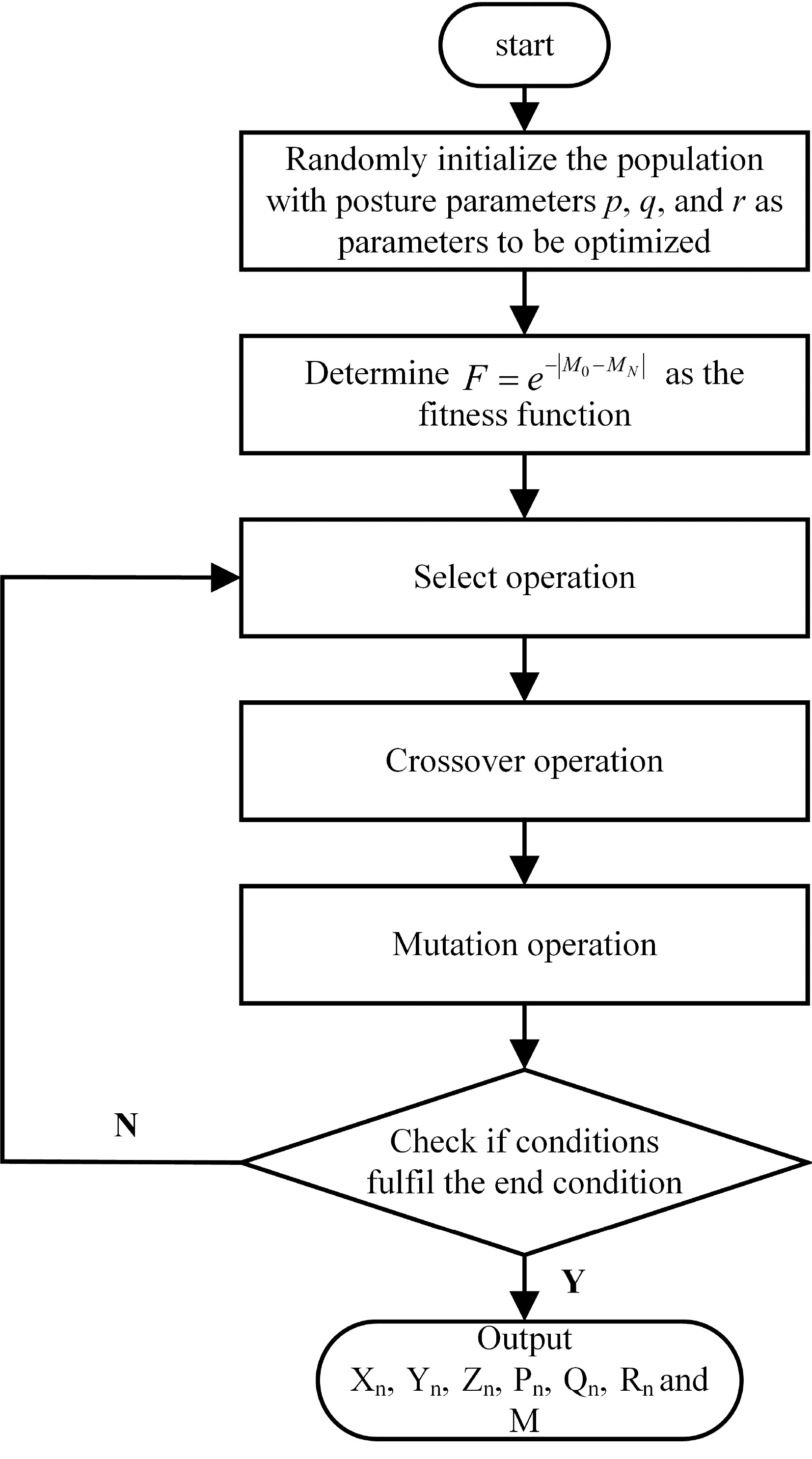
Figure 10.
Genetic algorithm optimization flow chart.
1) Randomly initialize the population: The individual coding is real-coded, with each individual constituting a real string composed of posture parameters (P, Q, R) of the coupling mechanism;
2) Determine the fitness function: To keep the mutual inductance in the misaligned state stable, the output of the mutual inductance surrogate model constructed, MN, and the target mutual inductance value, M0, are used to define the following fitness function:
$ F = {e^{ - \left| {{M_0} - {M_N}} \right|}} $ (16) 3) Select operation: Select a number of individuals from the population as parents for breeding offspring and use the roulette wheel selection method to select operations. Individuals with high fitness have higher probabilities of passing their parameters to the next generation; the converse is true for individuals with low fitness. The probability pd of individual d being selected is:
$ {p_d} = \dfrac{{{F_d}}}{{\displaystyle\sum\limits_{d = 1}^h {{F_d}} }} $ (17) where, h is the number of individuals in the population and Fd indicates the fitness value of individual d;
4) Crossover operation: Two paired individuals exchange some of their genes with the crossover probability p, thus forming two new individuals. Using the real-valued crossover method, the crossover method of the t-th gene of individuals s1 and s2 can be represented as:
$ \left\{ \begin{gathered} {g_{{s_1}t}} = {g_{{s_1}t}}r + {g_{{s_2}t}}(1 - r) \\ {g_{{s_2}t}} = {g_{{s_2}t}}r + {g_{{s_1}t}}(1 - r) \\ \end{gathered} \right. $ (18) where
$ {g_{{s_1}t}} $ $ {g_{{s_2}t}} $ 5) Mutation operation: To increase the diversity of the population, select the j-th gene gij of the i-th individual with a relatively small mutation probability ps to mutate. The mutation operation method is as follows:
Through the optimization algorithm proposed in this section, the posture parameters of the coupling mechanism for constant power transfer in the misaligned position can be accurately obtained.
$ {g_{i j}} = \left\{ \begin{gathered} {g_{i j}}{r_2} + ({g_{i j}} - {g_{\max }}){r_1}(1 - s/{s_{\max }}),\quad{r_2} \geqslant 0.5 \\ {g_{i j}}{r_2} + ({g_{\min }} - {g_{i j}}){r_1}(1 - s/{s_{\max }}),\quad{r_2} \lt 0.5 \\ \end{gathered} \right. $ (19) where gmax and gmin are the upper and lower bounds of gene gij, respectively, r1 is a random number, s is the current iteration number, smax is the maximum number of evolutions, and r2 is a random number between 0 and 1;
6) Check if the fitness function value fulfills the end condition: If the condition is met, output the optimization result; otherwise proceed with the next iteration.
Through the optimization algorithm proposed in this section, the posture parameters of the coupling mechanism for constant power transfer in the misaligned position can be accurately obtained.
-
To verify the accuracy of the algorithmic design and optimization process described in the previous section, in this chapter the optimization outcome of applying the algorithm to the lateral misalignment of the system when the distance-to-diameter ratio of the coupling mechanism is 0.6 is simulated. As the relative position parameters (x, y, z) of the primary and secondary coils during AUV wireless power transfer can be directly obtained from a sensor, the posture parameters (α, β, γ) of the secondary coil were optimized to maintain a constant mutual inductance at the misaligned position of the system. The reference point of the mutual inductance value when both coils are facing each other, M0 = 9.8265 µH, was set as the algorithm’s optimization target. Test points were taken along the misaligned path from one misaligned point (−50, 0, 60) to the other misaligned point (50, 0, 60) with a step length of 5 cm, resulting in a total of 21 test points to form the experimental set. The constant mutual inductance algorithm was optimized for the experimental set and the electromagnetic field simulation model was developed using the COMSOL finite element analysis software for simulation verification. The results of the optimization are shown in Fig. 11 below; the optimization results and raw error for each test point are listed in Table 7. Mutual inductance values before and after optimization of each test point in the experimental set are shown in Fig. 11.
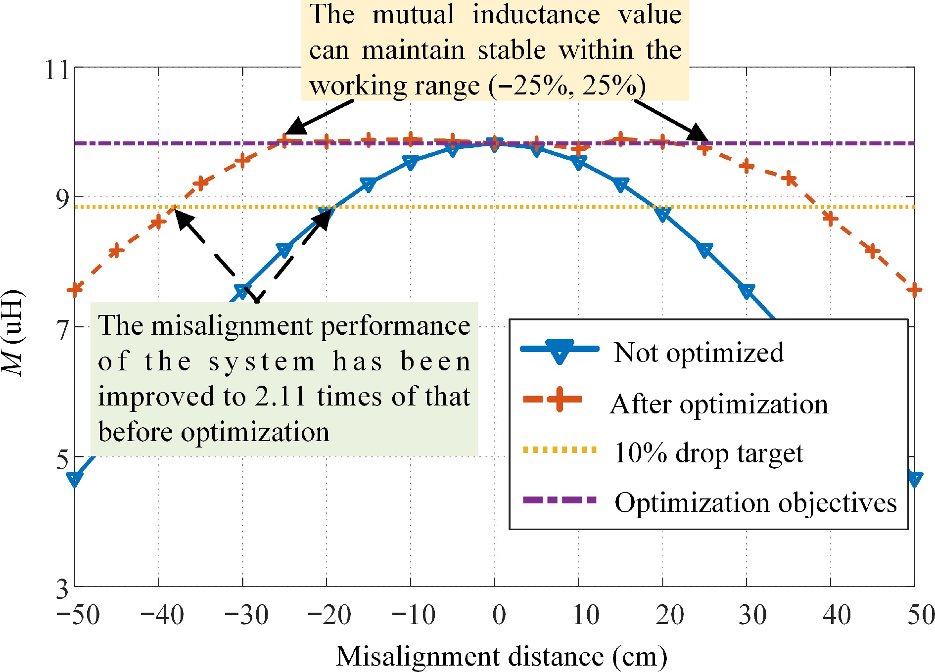
Figure 11.
Comparison of the mutual inductance of the system before and after optimization.
Table 7. Optimization results for each test point and error from the original data.
Misalignment distance (cm) Rotation angle p (around x-axis) Rotation angle q (around y-axis) Rotation angle r (around z-axis) Mutual inductance without optimization algorithm (µH) Mutual inductance with optimization algorithm (µH) Optimized target of mutual inductance (µH) Error (µH) –50 86.44 –84.27 –85.64 4.6686 7.5662 9.8265 2.2603 –45 –89.42 49.9 89.83 5.4052 8.1761 9.8265 1.6504 –40 60.22 –59.56 –56.96 6.1473 8.6204 9.8265 1.2061 –35 73.18 45.05 –89.47 6.8746 9.2045 9.8265 0.622 –30 60.15 –35.85 –85.09 7.5657 9.5580 9.8265 0.2685 –25 33.10 –52.27 –51.11 8.1992 9.8658 9.8265 –0.0393 –20 –39.71 –36.58 16.72 8.7536 9.8517 9.8265 –0.0252 –15 –27.41 –31.49 –5.61 9.2086 9.8773 9.8265 –0.0508 –10 –33.45 –11.05 –6.70 9.5472 9.8895 9.8265 –0.063 –5 24.69 30.02 –1.25 9.7558 9.8636 9.8265 –0.0371 0 0 0 0 9.8265 9.8265 9.8265 0 5 17.83 –42.31 49.78 9.7559 9.8213 9.8265 0.0052 10 47.24 –10.61 20.01 9.5472 9.7403 9.8265 0.0862 15 –8.23 59.41 –49.73 9.2086 9.8909 9.8265 –0.0644 20 0.65 50.41 –34.48 8.7534 9.8502 9.8265 –0.0237 25 –3.67 60.82 –31.31 8.1994 9.7524 9.8265 0.0741 30 –58.25 35.81 –87.47 7.5658 9.4767 9.8265 0.3498 35 77.82 29.26 84.01 6.8745 9.2901 9.8265 0.5364 40 85.82 48.16 88.63 6.147 8.6633 9.8265 1.1632 45 89.99 41.02 89.99 5.4055 8.1647 9.8265 1.6618 50 89.99 48.85 89.99 4.6687 7.5706 9.8265 2.2559 From the figure, it is seen that the optimization algorithm can effectively achieve a constant mutual inductance value within the working range of the coupling mechanism with a misalignment distance of up to 25%. For the 11 sampling points, the average absolute and maximum absolute errors were 0.0426 and 0.0862 µH, respectively, and the average and maximum relative errors were 0.43% and 0.88%, respectively.
Figure 12 shows convergence diagrams of the optimization algorithm for each test point within the working range. At each test point, convergence was achieved within 20 iterations, demonstrating that the proposed algorithm can achieve good convergence to the optimal value over a small number of iterations, indicating that it is practical and can be applied in UWPT systems.
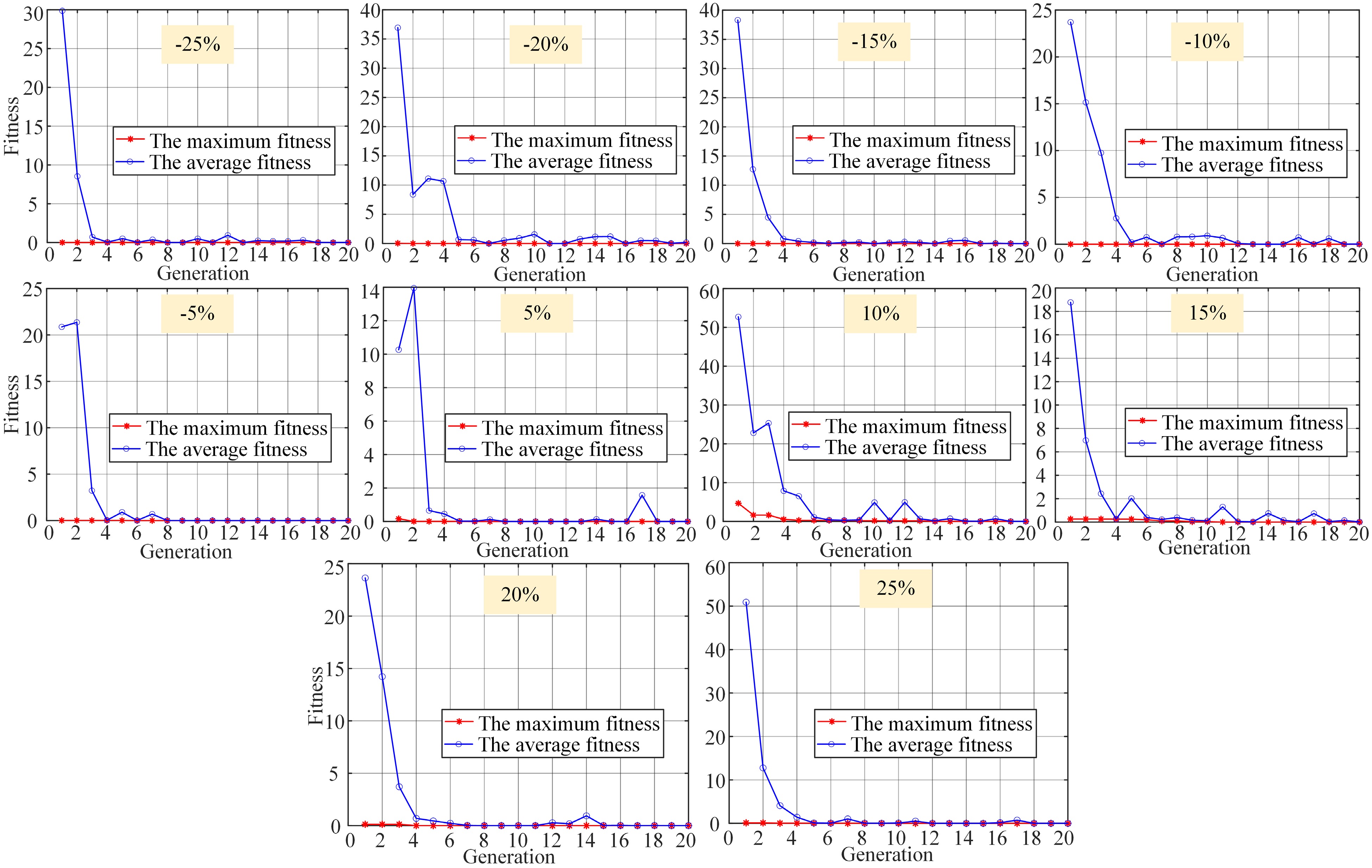
Figure 12.
Test set global optimization convergence process.
The posture and distribution of the magnetic field of the coupling mechanism at each misaligned point within the working range are shown in Fig. 13. When the misalignment distance exceeded 25%, the mutual inductance could not be stabilized by adjusting the posture of the secondary coil, causing an inevitable drop in the mutual inductance. However, even in this extreme case the proposed optimization algorithm was still effective in significantly improving the mutual inductance, as shown in Fig. 14. When the mutual inductance dropped, the average mutual inductance of the system increased by 40.33%, with a maximum increase of 62.16%.
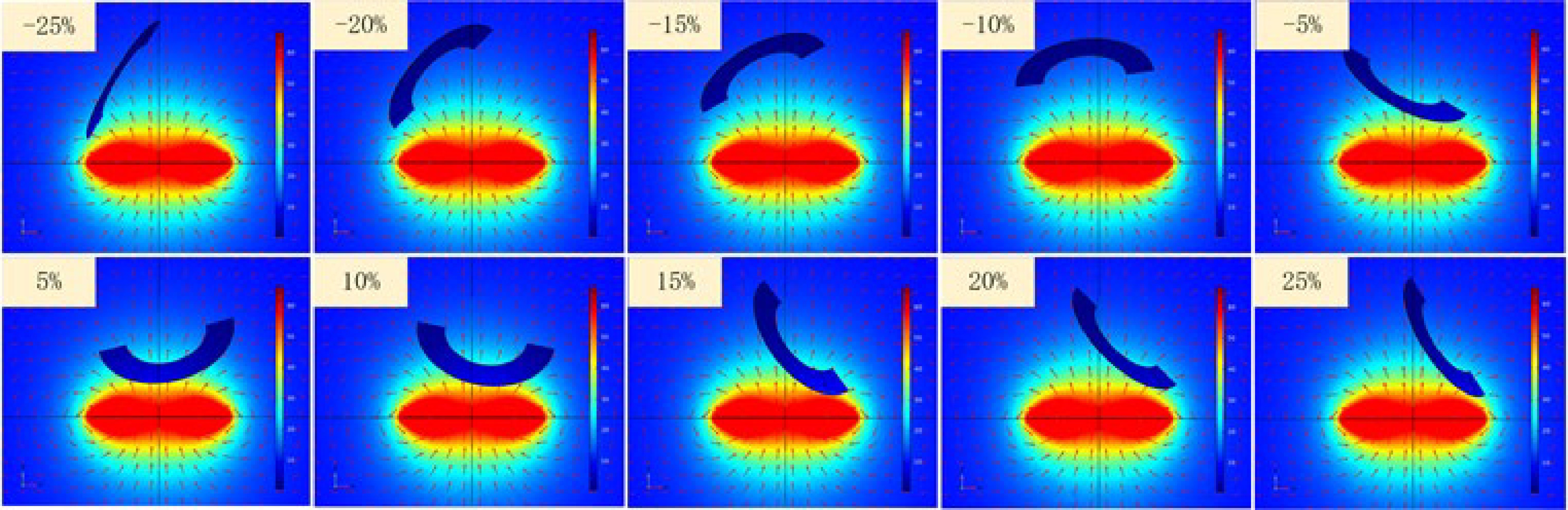
Figure 13.
Electromagnetic field simulation for each test point within the working range.
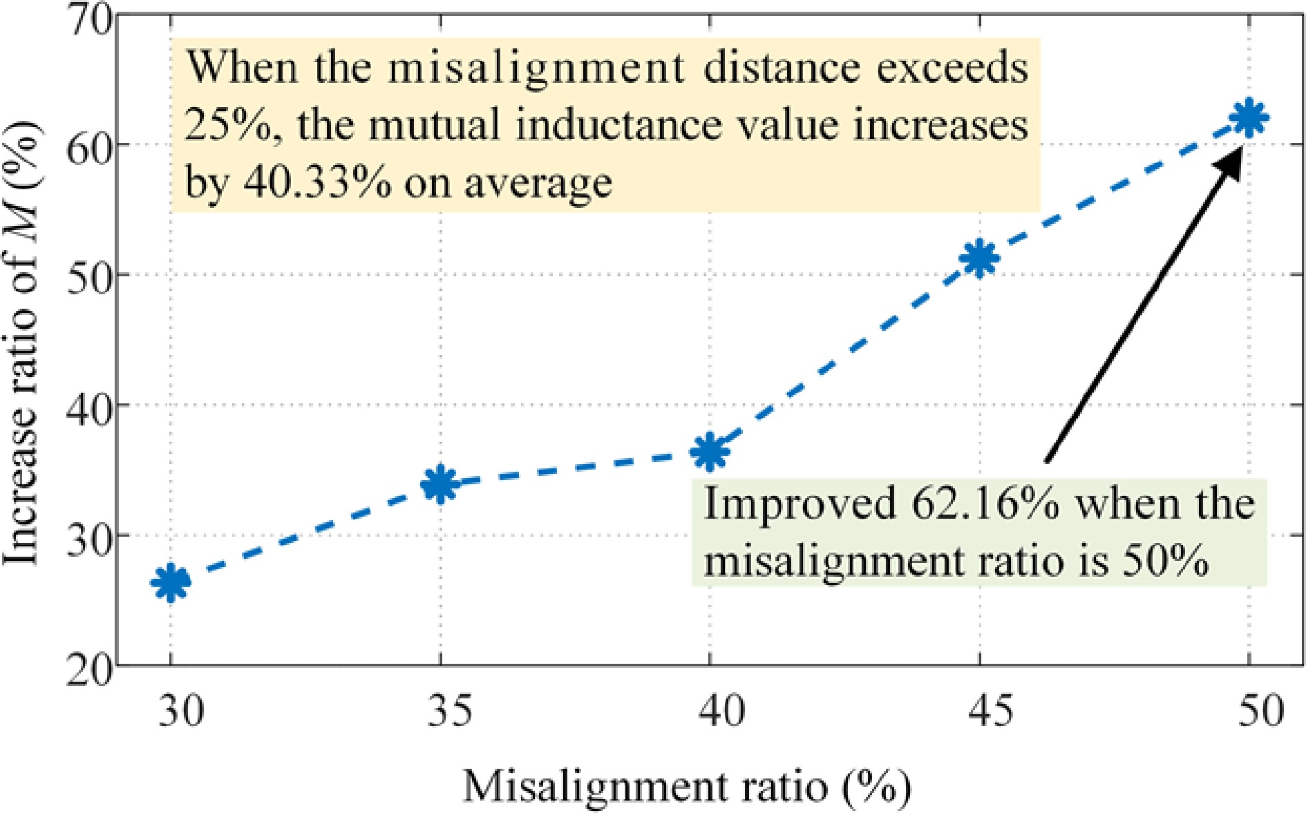
Figure 14.
Improvement of mutual inductance outside of the stable range by the optimization algorithm.
In practical applications, fluctuations in mutual inductance within a range of 10% can be resolved via control methods. Under such conditions, as shown in Fig. 11, the anti-misalignment performance of the system increased by a factor of 2.11 relative to a case in which the secondary coil posture was not changed during misalignment, thereby effectively alleviating the impact of the drop in mutual inductance on the system's power transfer characteristics in the misaligned state.
-
To further verify the practicality and accuracy of the algorithm design and optimization results, this section describes the experimental verification of the constant mutual inductance region of the mutual inductance curve of the experimental setup at a misalignment of between −25% and 25%. A 1 kW AUV wireless charging experimental prototype with LCC-S topology was established, as shown in Fig. 15. The full bridge inverter comprised four MOSFETs (NCEPOWER, NCE65T180F) driven by two half-bridge drivers (ST, L6387ED). The rectifier comprised four diodes (ONSEMI, MBR201000CT), and the main control chip adopted a complex programmable logic device (CPLD) (ALTERA, EPM240T100C5, with a crystal oscillator at 50 MHz). The system frequency, dead time, and system load were set to 152 kHz, 150 ns, and 20 Ω, respectively.
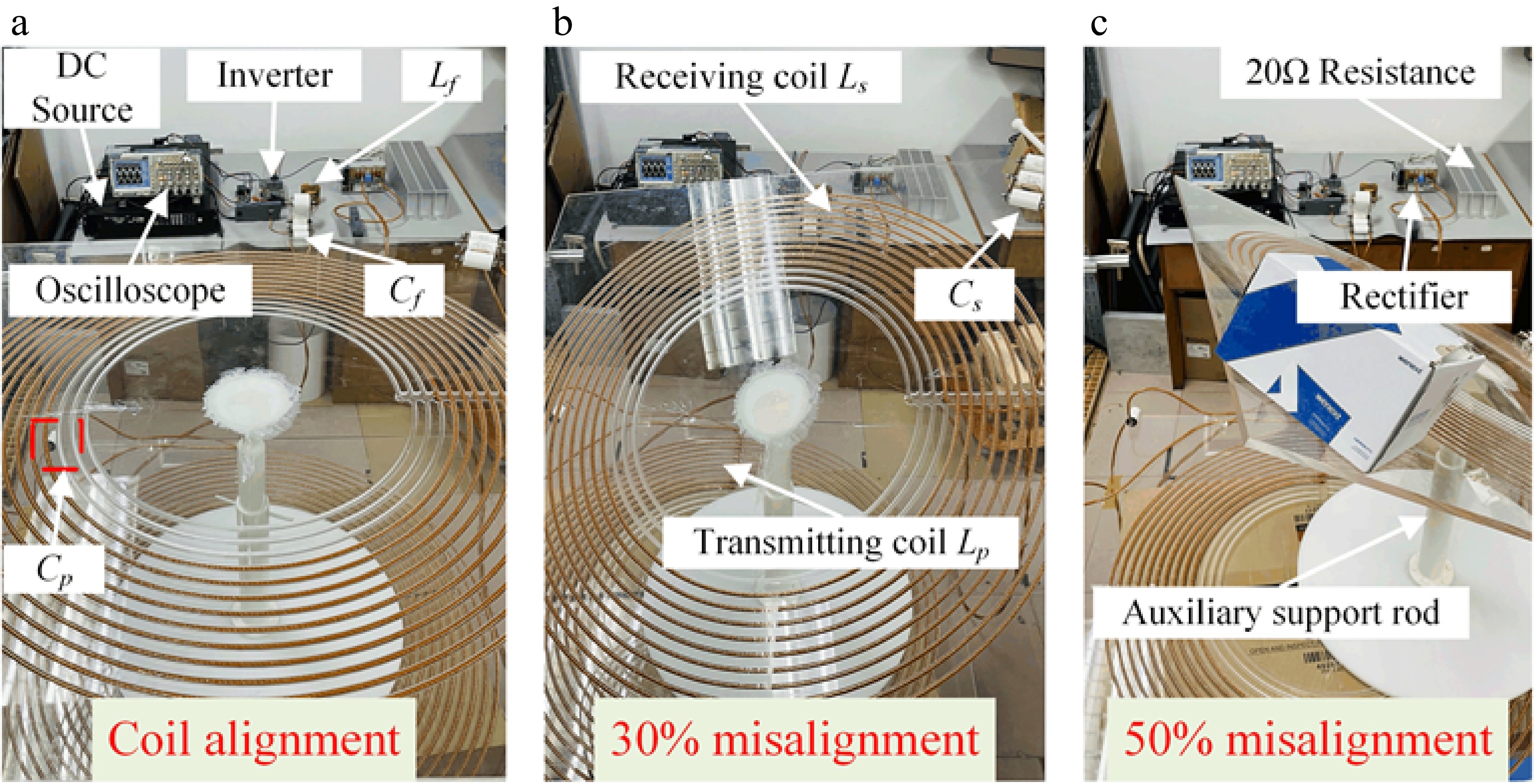
Figure 15.
Experimental prototype. (a) Coil alignment. (b) 30% misalignment. (c) 50% misalignment.
Verification of mutual inductance stability
-
From the theoretical analysis above, it was evident that mutual inductance would be a key factor in determining the power stability of the experimental system. Therefore, the stability of the mutual inductance was experimentally verified first. It was ensured that the primary and secondary coils were completely opposite, i.e., that the secondary coil had no misalignment or rotation and could serve as the reference point of the experiment. The secondary coil was also set as the optimization target of the experiment, with the mutual inductance value of the reference point measured as 10.7 µH. Furthermore, the simulation verification test points were used as the test points for the experimental verification and the misalignment pathway between the two misaligned points [(−50,0,60) and (50,0,60), respectively] was sampled with a step size of 5 cm. The measured mutual inductance values of each test point before and after optimization by the algorithm are shown in Fig. 16.
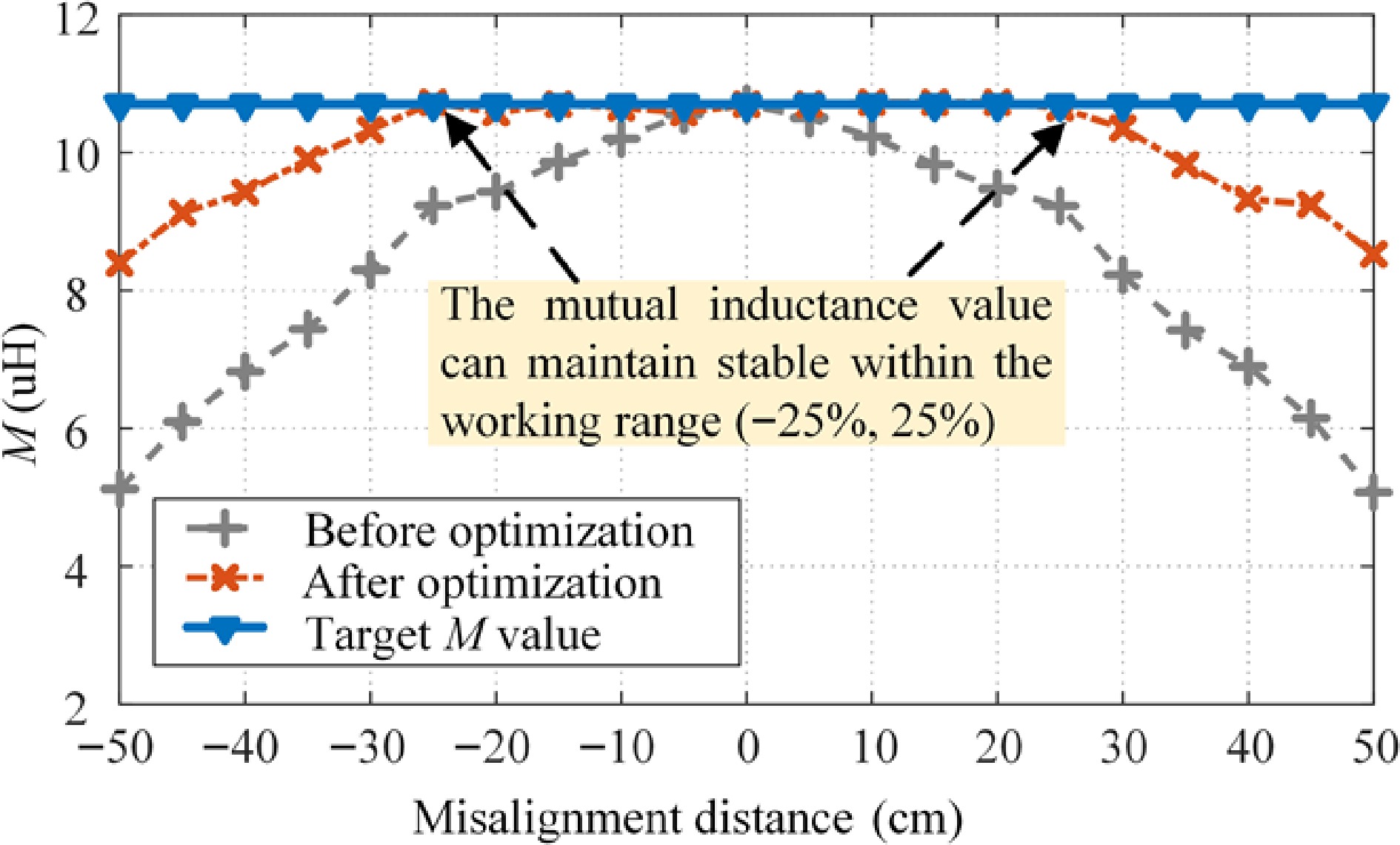
Figure 16.
Comparison curve for mutual inductance M.
Evidently, using the algorithm, the mutual inductance value of the coupling mechanism could be stabilized by adjusting the posture of the secondary coil within the working range (−25%, 25%) with an average error of 4.2%. The mutual inductance of the system also significantly improved beyond the working range, with a maximum increase of 63.9%, a result consistent with the simulation results.
Verification of power stability
-
To further verify the practicality of the proposed algorithm, a power experiment was performed on the experimental system at test points within the working range, with the different cases of resulting power transfer shown in Fig. 17. When the coupling mechanism was aligned, the power transfer of the system was 1,155.2 W with an efficiency of 91.2%. When the system was misaligned by 25%, the optimizing algorithm maintained the mutual inductance at around 10.6 µH with a system efficiency of 90.8%. Using the method proposed in this paper, the waveforms of the current and voltage of the system in misalignment situations were fundamentally unchanged, thereby confirming power stability. Furthermore, soft switching was attained over the full range of misalignment to ensure the safe and efficient operation of the system, maintaining the system efficiency at approximately 90%.
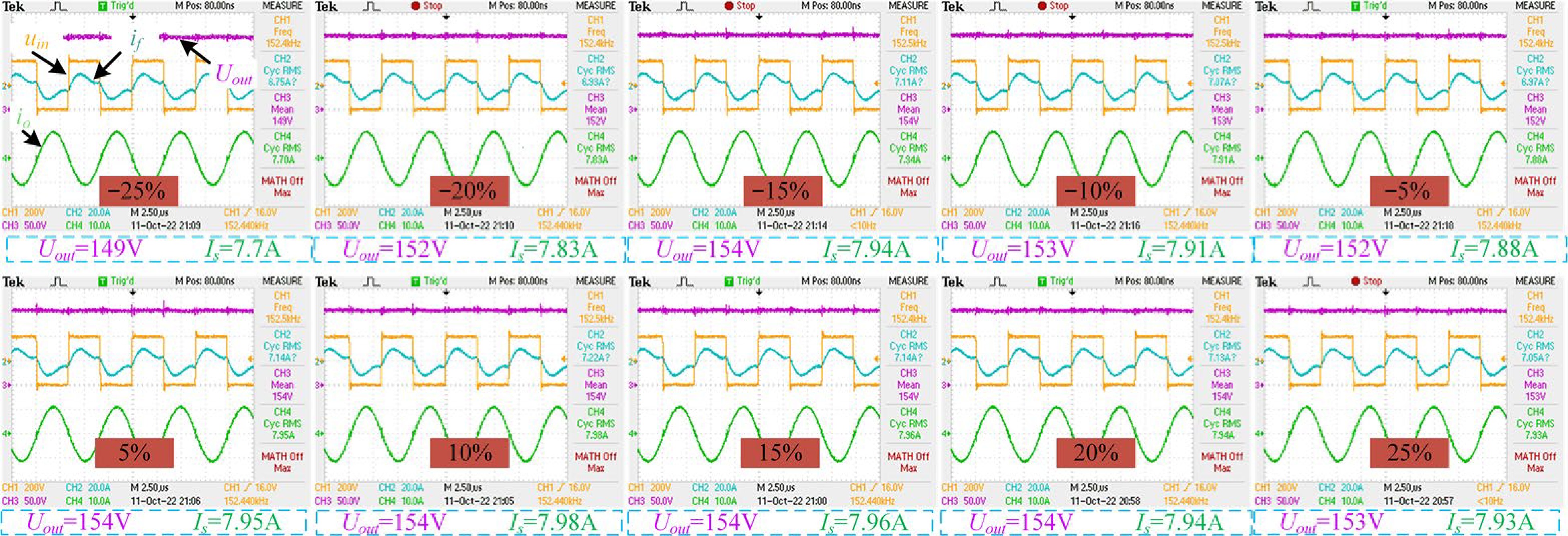
Figure 17.
Experimental waveforms for different misalignment cases with the proposed algorithm adopted.
Based on the power curve in Fig. 18, it is evident that the optimized system can perform a constant power transfer of 1.15 kW in the misaligned state. The overall efficiency of the system reached 91% and the average power transfer of the system increased by 18.91%, with a maximum increase of 48.16%. There was some deviation between the experimental and simulation reference points, primarily the result of deviations in the measurement of the experimental environment and system parameters. However, as the relative errors of the experiment were very small, the optimization algorithm proposed in this paper was shown to be accurate and effective.
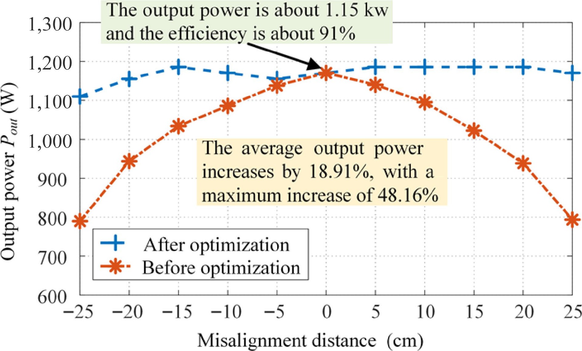
Figure 18.
Comparison curve for output power Pout.
-
This paper proposed an optimal misalignment posture prediction algorithm for coupling mechanisms based on the mutual inductance surrogate model. The algorithm predicts the optimal posture for constant power transfer in the misaligned state of a coupling mechanism within its working range by adjusting the posture of the secondary coupling mechanism. The simulation and experimental results reported in this paper indicate that the proposed algorithm can achieve constant mutual inductance, thereby ensuring constant power transfer. Unlike existing anti-misalignment solutions used by the wireless power transfer systems of AUV, the proposed algorithm avoids issues with docking and reduces the structural complexities of the wireless charging coupling mechanism, enabling dynamic wireless charging underwater and significantly enhancing flexibility and practicality.
The strengths and significance of the research reported in this paper can be enumerated as follows: (1) The constructed surrogate model can accurately derive the mutual inductance value of a coupling mechanism at any position and posture. (2) The optimization algorithm proposed in this paper can effectively achieve a constant mutual inductance value in a coupling mechanism in the misaligned state in 3D space, thereby achieving stable power transfer. (3) The method proposed in this paper can be adapted to other fields and is not limited by the elements constituting the coupling mechanism in terms of shape, material, or the presence or absence of a magnetic core. The experimental prototype was built to verify the practicality of the proposed method revealed that the system can guarantee a constant mutual inductance within a 25% misalignment range and an aspect ratio of 0.6 with an average error of only 4.2%. When the mutual inductance falls within 10%, the anti-misalignment range of the system is increased to 2.11 times that before optimization.
-
The roles and contributions to the paper of each author are described as follows: Study conception and design: Feng Y, Sun Y; data collection: Feng Y, Lin T, Chen F; analysis and interpretation of results: Feng Y, Hu H; draft manuscript preparation: Feng Y. All authors reviewed the results and approved the final version of the manuscript.
-
All data included in this study are available upon request by contact with the corresponding author.
This work was supported by the Fundamental Research Funds for the Central Universities under Grant 2022CDJQY-006, and the National Natural Science Foundations of China under Grant 62073047.
-
The authors declare that they have no conflict of interest.
- Copyright: © 2024 by the author(s). Published by Maximum Academic Press, Fayetteville, GA. This article is an open access article distributed under Creative Commons Attribution License (CC BY 4.0), visit https://creativecommons.org/licenses/by/4.0/.
-
About this article
Cite this article
Feng Y, Sun Y, Lin T, Hu H, Chen F. 2024. Mutual inductance surrogate model of the UWPT system and its constant power optimization at misaligned positions. Wireless Power Transfer 11: e001 doi: 10.48130/wpt-0024-0001 

Mutual inductance surrogate model of the UWPT system and its constant power optimization at misaligned positions
- Received: 27 February 2024
- Revised: 25 March 2024
- Accepted: 15 April 2024
- Published online: 27 May 2024
Abstract: Recent studies have focused on developing underwater wireless power transfer (UWPT) anti-misalignment methods to address the vulnerability of UWPT systems to large water flow fluctuations and unstable power transference. Autonomous underwater vehicles (AUVs) use irregular coupling mechanisms to ensure stable power transmission through constant mutual inductance, but these require complex structures and present docking difficulties. A prediction algorithm based on the mutual inductance surrogate model is proposed to achieve optimal prediction for coupling mechanisms with constant power transmission at misaligned positions. The relative position and posture parameters of a coupling mechanism simulation model were subjected to Latin hypercube sampling to construct a dataset. Subsequently, a back propagation (BP) neural network was applied to develop an omnidirectional surrogate coupling mechanism model to predict the mutual inductance value. The surrogate model and a genetic algorithm were used to optimize the coil posture for maintaining constant power transfer. Experimental validation reveals that at a 0.6 aspect ratio, the system can ensure constant mutual inductance and power within a 25% omnidirectional misalignment range with an average error in mutual inductance of only 0.43%. At a 10% acceptable mutual inductance drop threshold, the anti-misalignment ranges of the system increase to 2.11 times the pre-optimization range.
-
Key words:
- WPT /
- Surrogate model /
- Machine learning