Building trust for traffic flow forecasting components in intelligent transportation systems via interpretable ensemble learning

Jishun Ou; Jingyuan Li; Chen Wang; Yun Wang; Qinghui Nie; Jishun Ou; Jingyuan Li; Chen Wang; Yun Wang; Qinghui Nie

doi:10.48130/dts-0024-0012

Figures (8) Tables (7)

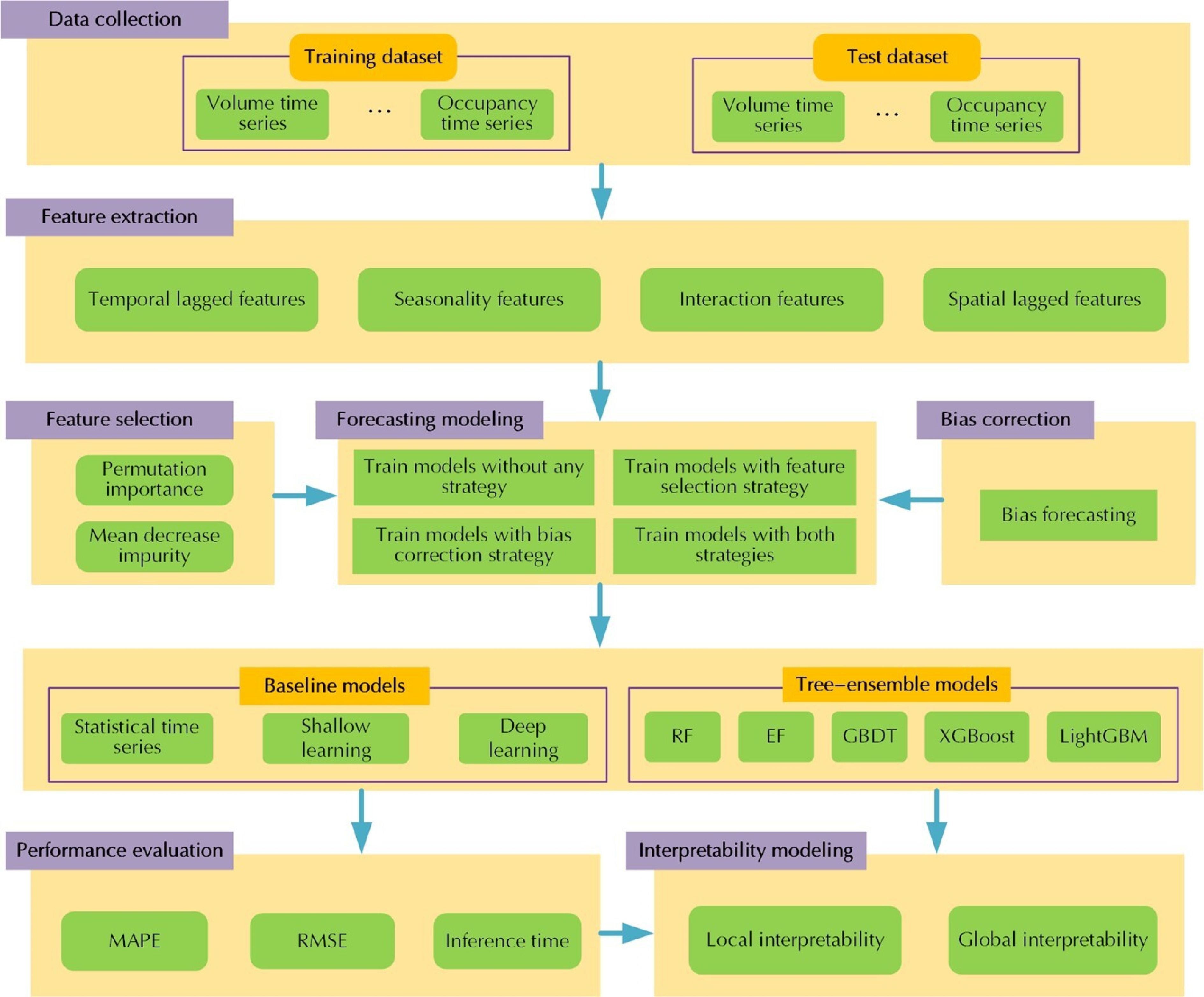
Figure 1.
The proposed interpretable traffic flow forecasting framework.
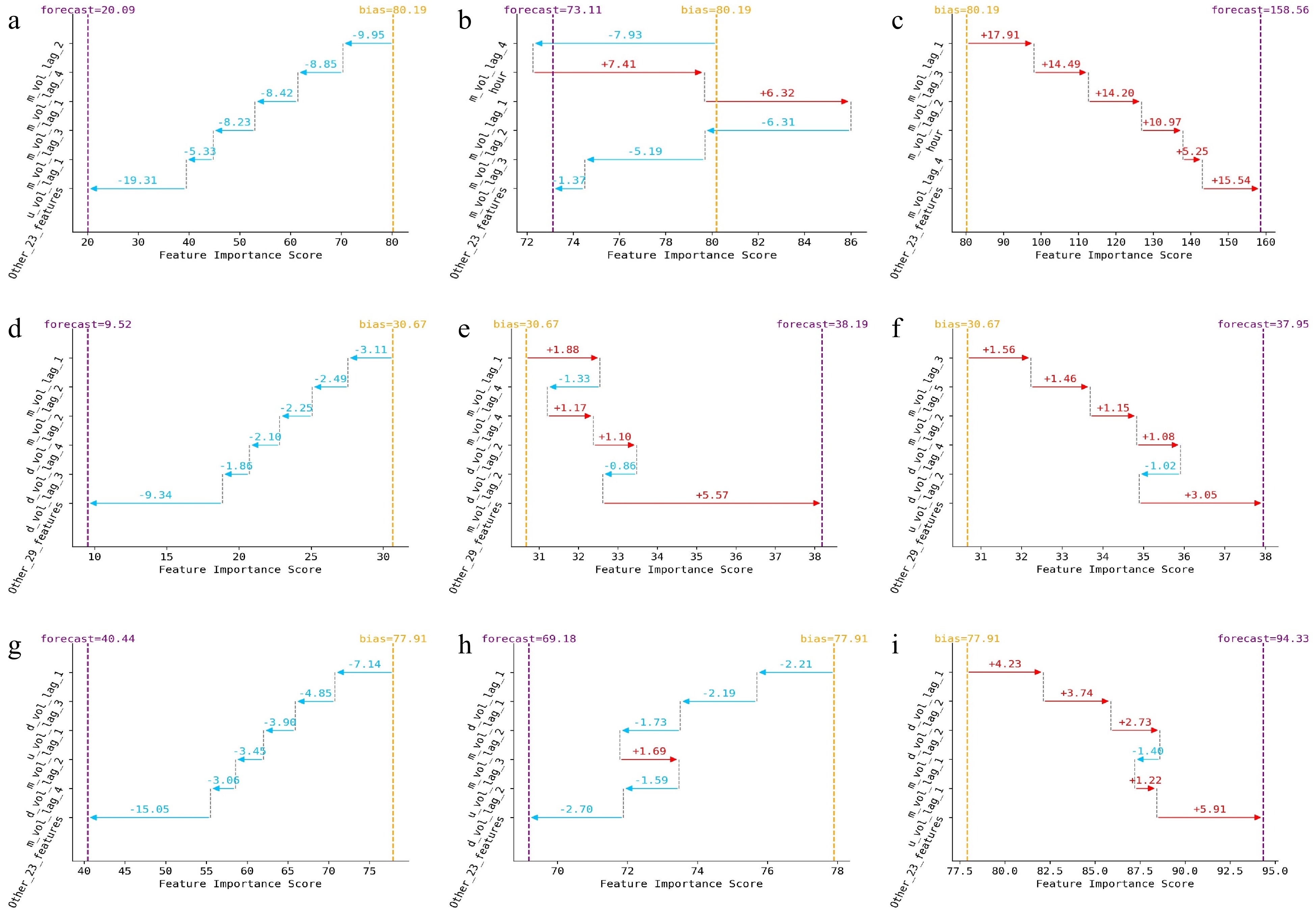
Figure 2.
Local model explanations using decision path plots for different traffic flow instances. Arterial instance at (a) 5:30 am, (b) 6:30 am, (c) 7:30 am. Expressway instance at (d) 5:30 am, (e) 7:30 am, (f) 8:00 am. Freeway instance at (g) 5:30 am, (h) 6:30 am, (i) 7:30 am.
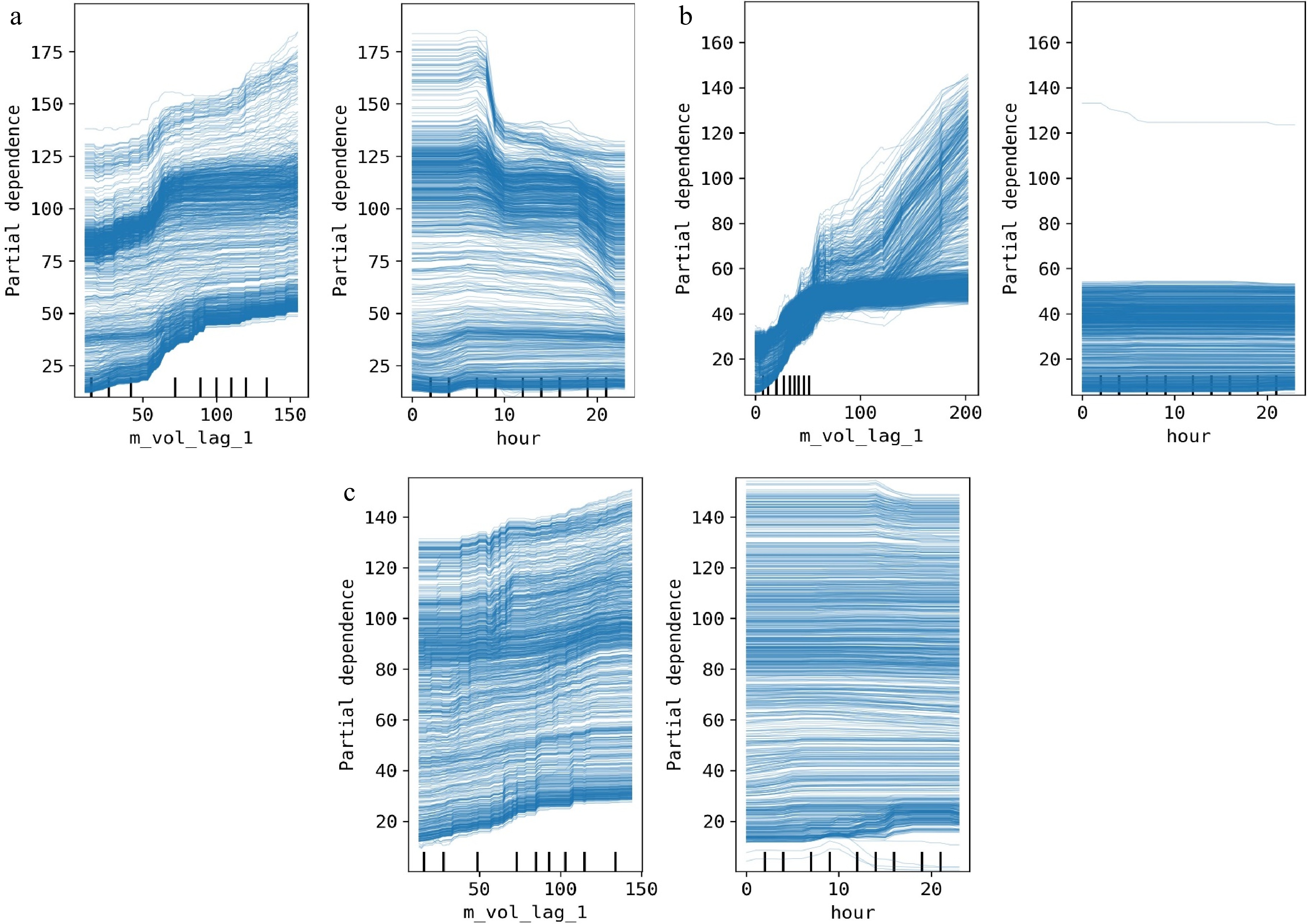
Figure 3.
Local model explanations using ICE plots for different traffic flow datasets. (a) Arterial dataset, (b) expressway dataset, (c) freeway dataset.
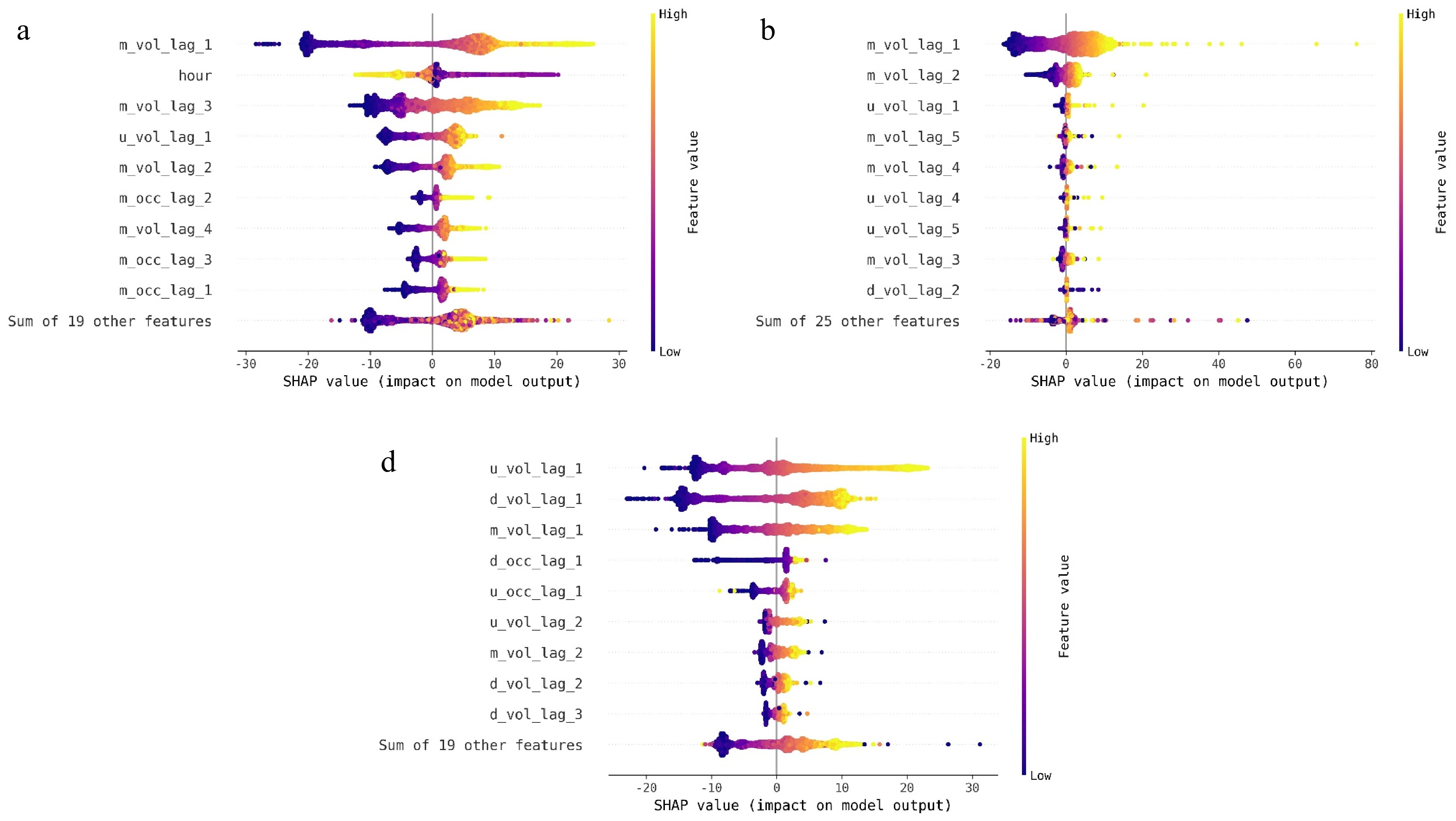
Figure 4.
Local model explanations using beeswarm plots for different traffic flow datasets. (a) Arterial dataset, (b) expressway dataset, (c) freeway dataset.
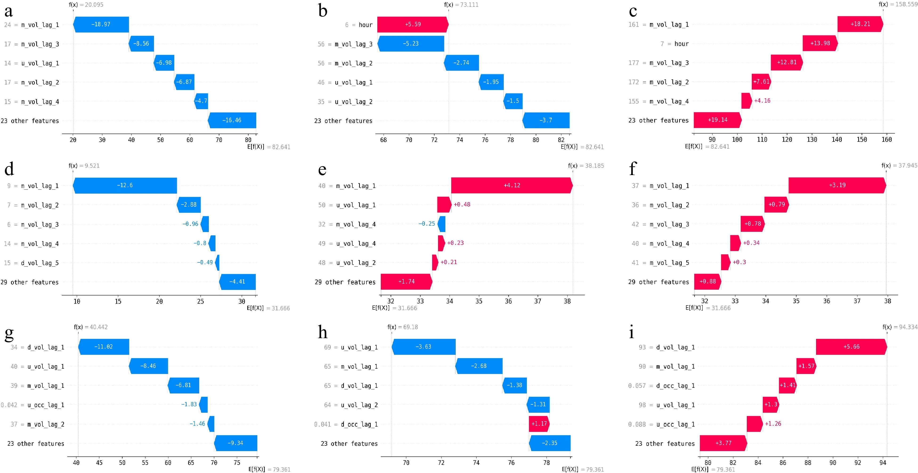
Figure 5.
Local model explanations using waterfall plots for different traffic flow instances. (a) Arterial instance at (a) 5:30 am, (b) 6:30 am, (c) 7:30 am. Expressway instance at (d) 5:30 am, (e) 7:30 am, (f) 8:00 am. Freeway instance at (g) 5:30 am, (h) 6:30 am, (i) 7:30 am.
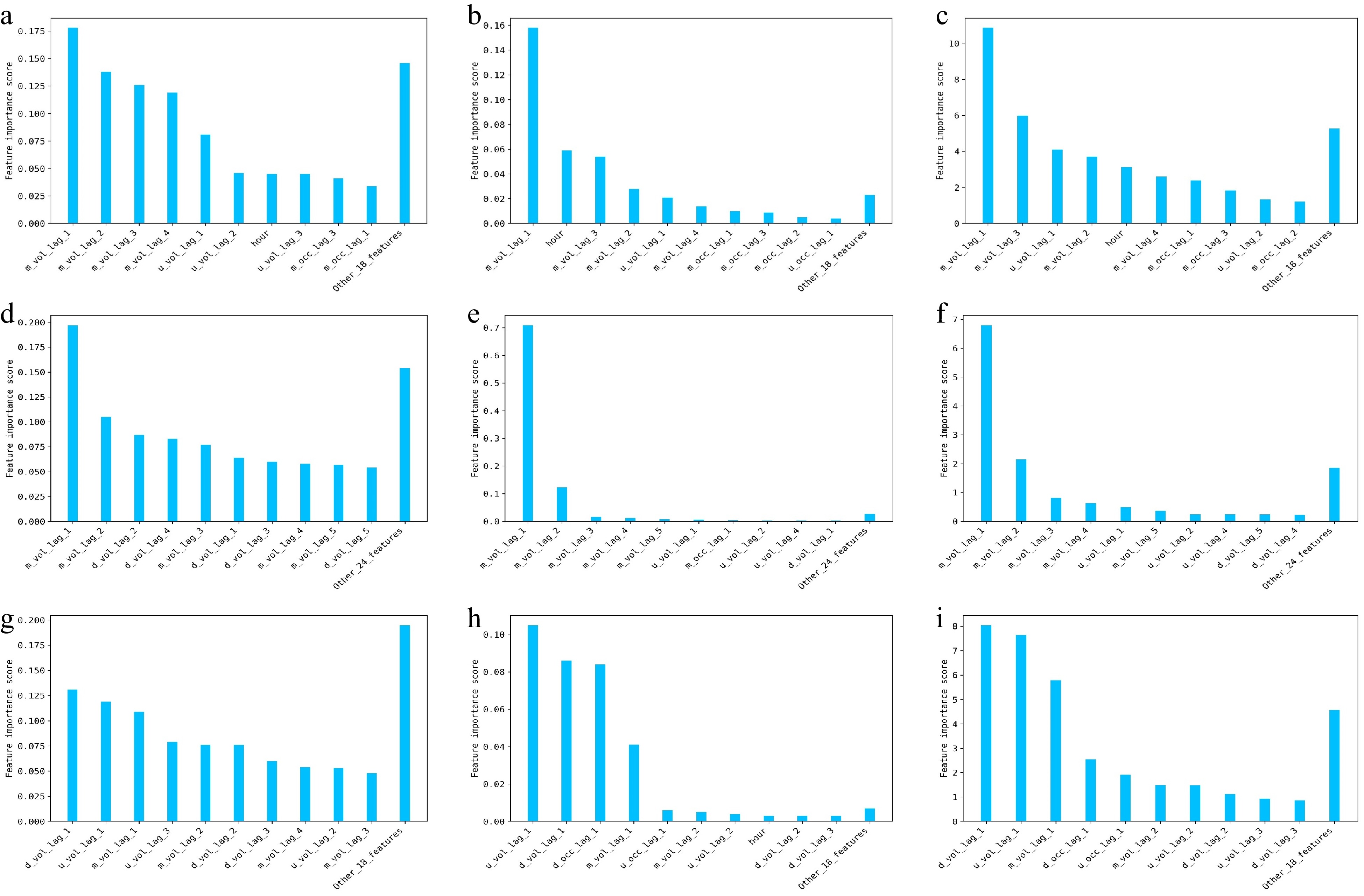
Figure 6.
Global model explanations using global feature importance methods for different traffic flow datasets. (a) MDI / arterial dataset, (b) PI / arterial dataset, (c) SHAP / arterial dataset, (d) MDI / expressway dataset, (e) PI / expressway dataset, (f) SHAP / expressway dataset, (g) MDI / freeway dataset, (h) PI / freeway dataset, (i) SHAP / freeway dataset.
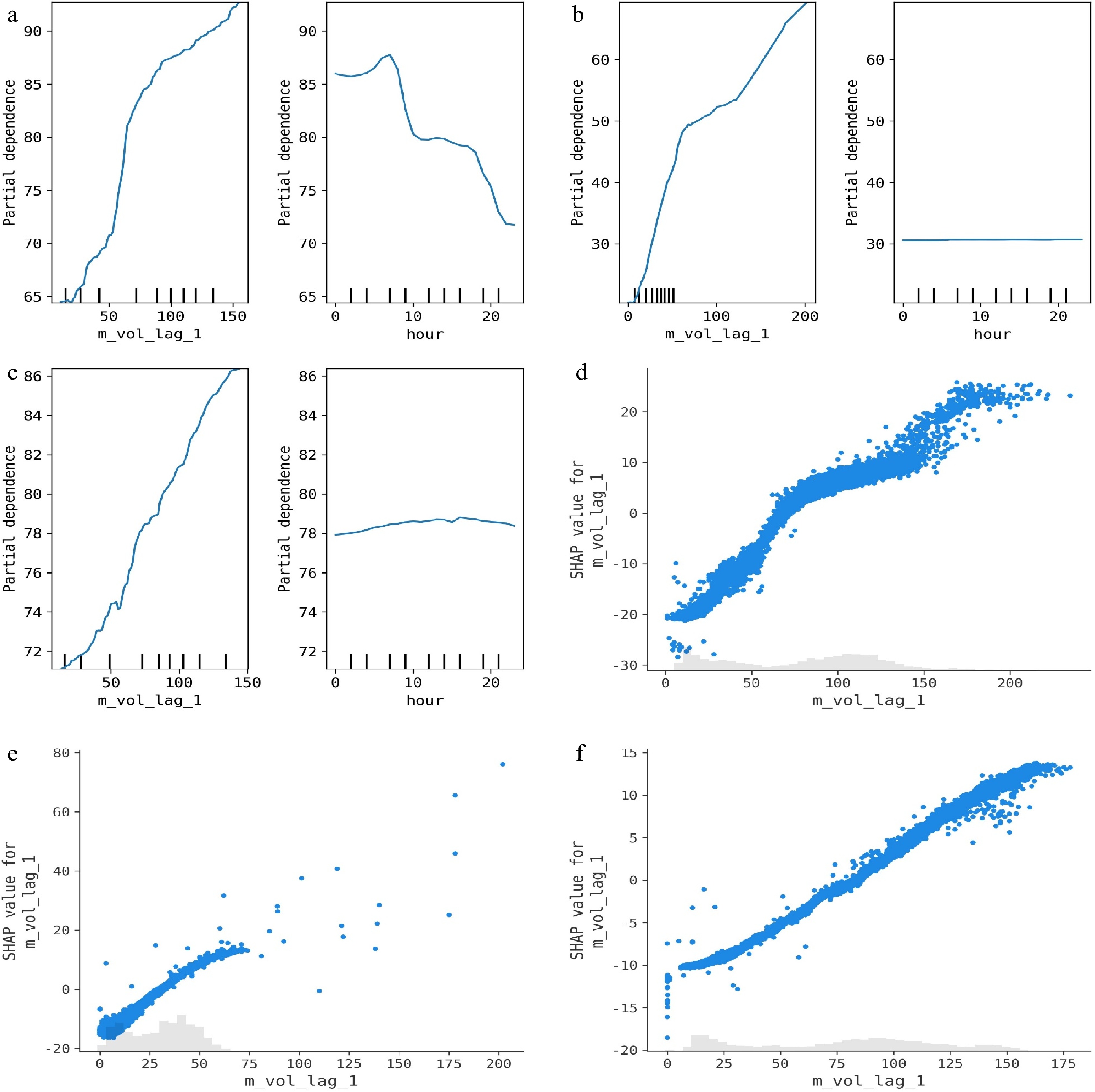
Figure 7.
Global model explanations using feature dependence plots for different traffic flow datasets. (a) 1D-PDP / arterial dataset, (b) 1D-PDP / expressway dataset, (c) 1D-PDP / freeway dataset, (d) SHAP dependence plot / arterial dataset, (e) SHAP dependence plot / expressway dataset, (f) SHAP dependence plot / freeway dataset.
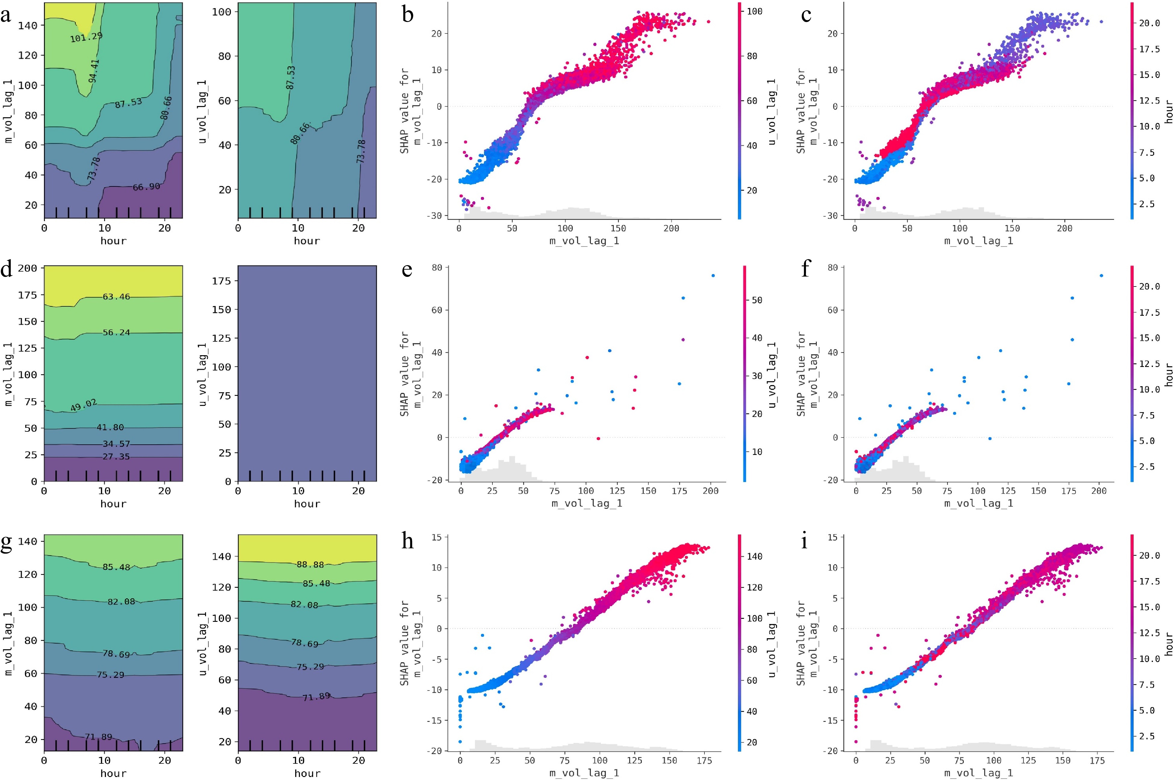
Figure 8.
Global model explanations using feature interaction effect plots for different traffic flow datasets. (a) 2D-PDP / arterial dataset, (b) SHAP interaction plot-1 / arterial dataset, (c) SHAP interaction plot-2 / arterial dataset, (d) 2D-PDP / expressway dataset, (e) SHAP interaction plot-1 / expressway dataset, (f) SHAP interaction plot-2 / expressway dataset, (g) 2D-PDP / freeway dataset, (h) SHAP interaction plot-1 / freeway dataset, (i) SHAP interaction plot-2 / freeway dataset.

City	Road type	Time interval	Total dataset size	Training set size	Test set size
Kunshan	Arterial	5-min	8064	6048	2016
Beijing	Expressway	2-min	40320	30240	10080
Seattle	Freeway	5-min	24192	18144	6048

Table 1.

Collected dataset information for traffic flow forecasting.

Model type	Models
Statistical time series	Autoregressive Integrated Moving Average (ARIMA)
Shallow learning	K-Nearest Neighbors (KNN), Linear Regression (LR), Least Absolute Shrinkage and Selection Operator (LASSO), Ridge Regression (RR), Regression Tree (RT), Extra Tree (ET)
Deep learning	LSTNET^[63], DeepAR^[64], NBEATS^[65], RNN, Transformer^[66]
Ensemble learning	RF, EF, GBDT, XGBoost, LightGBM

Table 2.

Developed traffic flow forecasting models.

Model type	Model	Arterial		Expressway		Freeway
Model type	Model	RMSE (veh/5-min)	MAPE (%)	RMSE (veh/2-min)	MAPE (%)	RMSE (veh/5-min)	MAPE (%)
Statistical time series	ARIMA	13.54	18.04	6.63	24.02	7.05	10.62
Shallow learning	KNN	13.12	16.06	6.91	23.30	6.68	10.58
	LR	13.62	17.91	6.53	22.12	6.46	10.30
	LASSO	13.65	18.04	6.55	23.54	6.59	10.28
	RR	13.62	17.97	6.54	22.12	6.45	10.39
	RT	14.31	17.46	7.60	25.70	7.27	10.97
	ET	14.37	17.38	6.86	24.59	7.60	13.22
Deep learning	LSTNET	13.41	17.01	6.56	21.60	6.95	10.23
	DeepAR	13.45	16.24	6.57	21.49	7.00	11.68
	NBEATS	13.79	16.18	6.55	21.37	6.12	10.49
	RNN	27.74	49.24	6.83	22.80	19.34	48.63
	Transformer	13.03	16.73	6.40	22.51	6.25	10.97
Ensemble learning	RF	12.42	15.60	6.49	23.29	6.28	9.44
	EF	12.35	15.80	6.31	24.06	6.28	9.70
	GBDT	12.28	15.81	6.34	22.79	5.94	9.61
	XGBoost	12.99	15.97	6.45	22.90	6.05	9.65
	LightGBM	12.39	16.06	6.27	22.74	5.96	10.55

Table 3.

Performance comparison of the developed models.

Model type	Model	Test time (s)
Model type	Model	Arterial	Expressway	Freeway
Statistical time series	ARIMA	0.12	0.13	0.11
Shallow learning	KNN	0.04	0.57	0.26
	LR	0.01	0.03	0.02
	LASSO	0.01	0.03	0.02
	RR	0.01	0.03	0.02
	RT	0.01	0.02	0.01
	ET	0.00	0.02	0.01
Deep Learning	LSTNET	37.84	187.67	151.25
	DeepAR	102.89	538.55	426.07
	NBEATS	42.70	217.81	175.83
	RNN	36.25	189.02	147.03
	Transformer	43.06	266.79	181.91
Ensemble Learning	RF	0.02	0.07	0.08
	EF	0.03	0.07	0.06
	GBDT	0.02	0.03	0.03
	XGBoost	0.01	0.02	0.02
	LightGBM	0.01	0.02	0.02

Table 4.

Test time of the developed models.

Developed models	Arterial				Expressway				Freeway
Developed models	RMSE (veh/5-min)	Trend	MAPE (%)	Trend	RMSE (veh/2-min)	Trend	MAPE (%)	Trend	RMSE (veh/5-min)	Trend	MAPE (%)	Trend
RF	12.40	↓	15.55	↓	6.49	→	22.70	↓	6.04	↓	9.18	↓
EF	12.03	↓	15.29	↓	6.23	↓	22.19	↓	5.95	↓	9.25	↓
GBDT	12.33	↑	15.56	↓	6.32	↓	22.43	↓	5.92	↓	9.56	↓
XGBoost	12.96	↓	15.86	↓	6.48	↑	22.91	↑	6.02	↓	9.52	↓
LightGBM	12.36	↓	15.77	↓	6.25	↓	22.25	↓	5.94	↓	10.41	↓

Table 5.

Performance comparison of the developed tree-ensemble models using the bias correction strategy.

Model	Feature selection measure	Arterial				Expressway				Freeway
Model	Feature selection measure	RMSE (veh/5-min)	Trend	MAPE (%)	Trend	RMSE (veh/2-min)	Trend	MAPE (%)	Trend	RMSE (veh/5-min)	Trend	MAPE (%)	Trend
RF	MDI	12.73	↑	16.02	↑	6.49	→	23.30	↑	6.75	↑	10.36	↑
	PI	12.67	↑	16.01	↑	6.49	→	23.30	↑	6.77	↑	10.37	↑
EF	MDI	12.49	↑	15.90	↑	6.38	↑	24.31	↑	6.50	↑	10.35	↑
	PI	12.45	↑	15.88	↑	6.44	↑	24.11	↑	6.73	↑	10.18	↑
GBDT	MDI	12.40	↑	15.91	↑	6.44	↑	23.20	↑	6.46	↑	9.96	↑
	PI	12.22	↓	15.89	↑	6.66	↑	23.93	↑	6.13	↑	9.33	↓
XGBoost	MDI	12.76	↓	15.87	↓	6.43	↓	22.88	↓	6.43	↑	10.11	↑
	PI	12.70	↓	16.01	↑	6.71	↑	22.80	↓	6.67	↑	10.17	↑
LightGBM	MDI	12.25	↓	15.74	↓	6.29	↑	22.55	↓	5.98	↑	10.26	↓
	PI	12.57	↑	16.07	↑	6.47	↑	23.69	↑	6.71	↑	10.50	↓

Table 6.

Performance comparison of different tree-ensemble models using the feature selection strategy.

Model	Feature selection measure	Arterial				Expressway				Freeway
Model	Feature selection measure	RMSE (veh/5-min)	Trend	MAPE (%)	Trend	RMSE (veh/2-min)	Trend	MAPE (%)	Trend	RMSE (veh/5-min)	Trend	MAPE (%)	Trend
RF	MDI_BC	12.58	↑	15.94	↑	6.49	→	23.24	↓	6.72	↑	10.42	↑
	PI_BC	12.58	↑	15.95	↑	6.49	→	23.24	↓	6.75	↑	10.41	↑
EF	MDI_BC	12.19	↓	15.46	↓	6.36	↑	23.20	↓	6.47	↑	10.16	↑
	PI_BC	12.18	↓	15.29	↓	6.40	↑	22.97	↓	6.67	↑	10.09	↑
GBDT	MDI_BC	12.37	↑	15.70	↓	6.43	↑	22.76	↑	6.43	↑	9.84	↑
	PI_BC	12.22	↓	15.57	↓	6.65	↑	23.11	↑	6.11	↑	9.18	↓
XGBoost	MDI_BC	13.01	↑	15.93	↓	6.48	↑	22.92	↑	6.45	↑	10.14	↑
	PI_BC	12.22	↓	16.01	↑	6.75	↑	22.90	→	6.68	↑	10.15	↑
LightGBM	MDI_BC	12.29	↓	15.51	↓	6.27	→	22.14	↓	5.96	→	10.09	↓
	PI_BC	12.58	↑	15.89	↓	6.47	↑	23.20	↑	6.71	↑	10.29	↓

Table 7.

Performance comparison of different tree-ensemble models using the bias correction and feature selection strategies.