-

Figure 1.
The schematics of lane-changing.
-
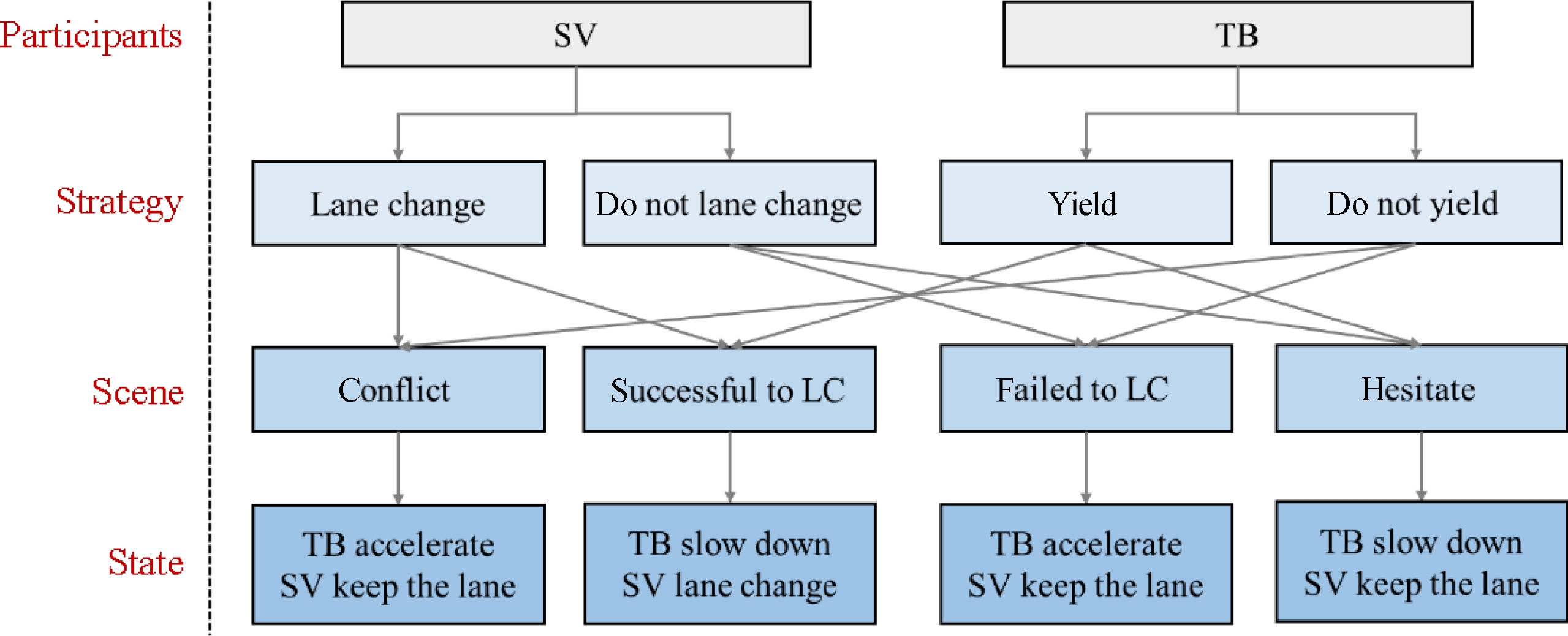
Figure 2.
The game process of the lane-changing decision.
-
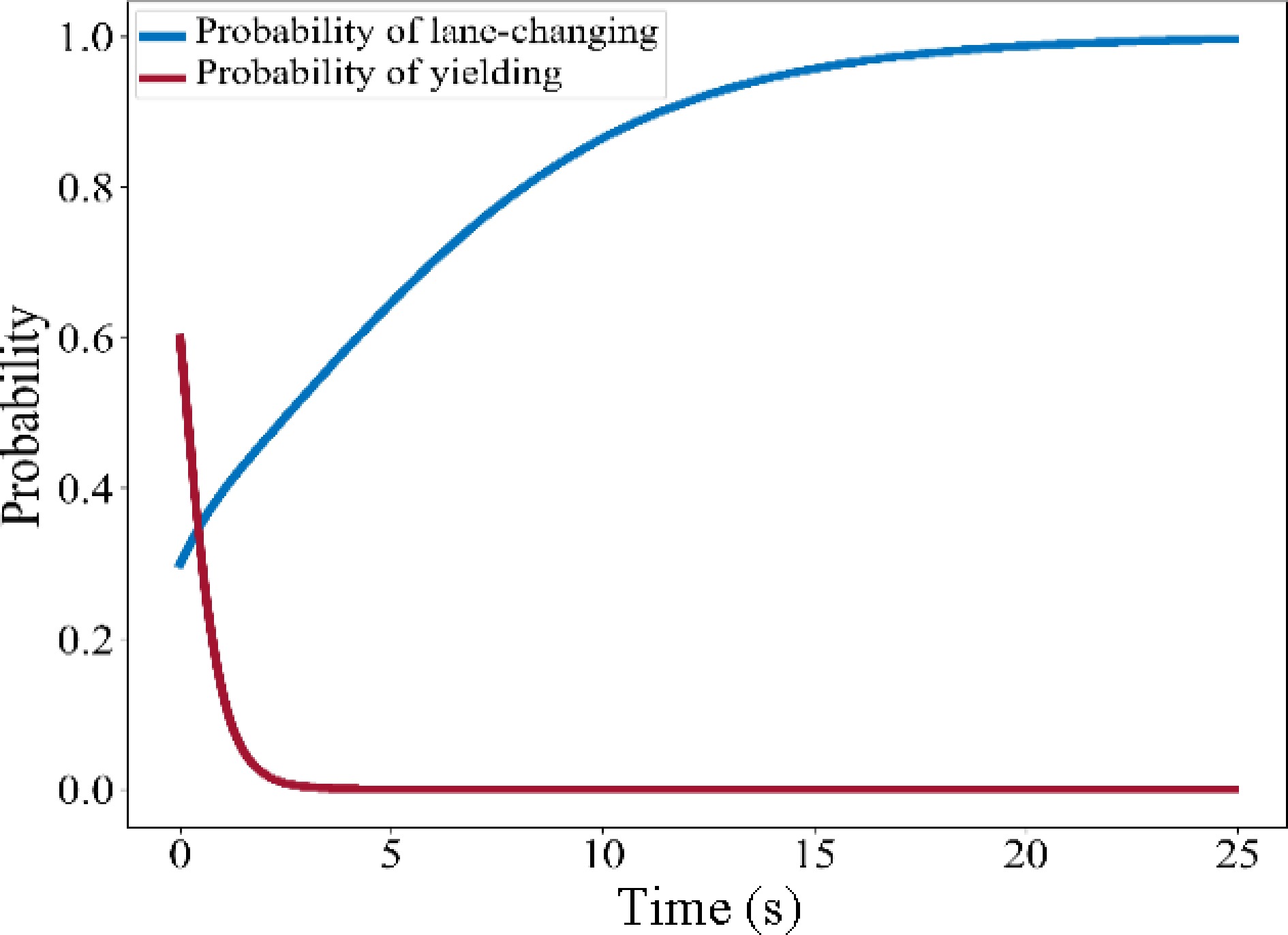
Figure 3.
Schematic diagram of the evolution of the probability.
-
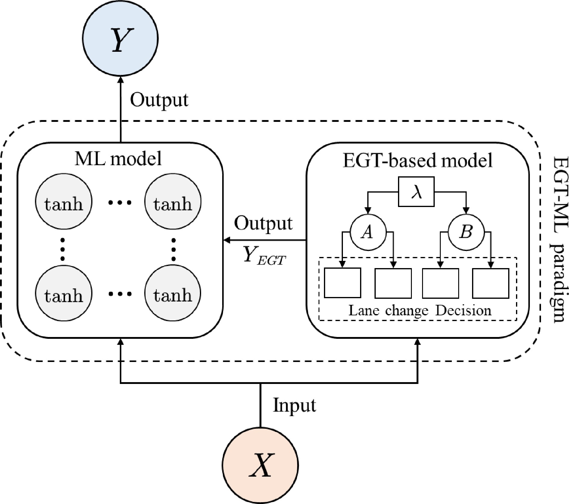
Figure 4.
Structure diagram of EGTML.
-
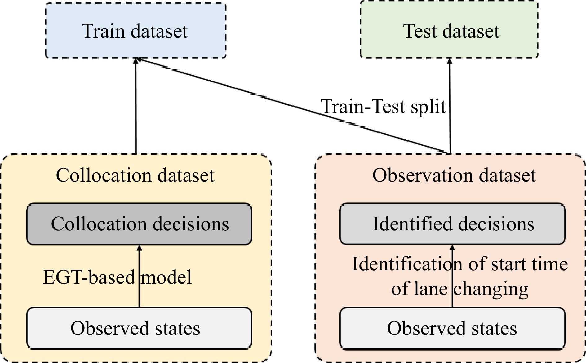
Figure 5.
Relationship between observation and collocation dataset.
-
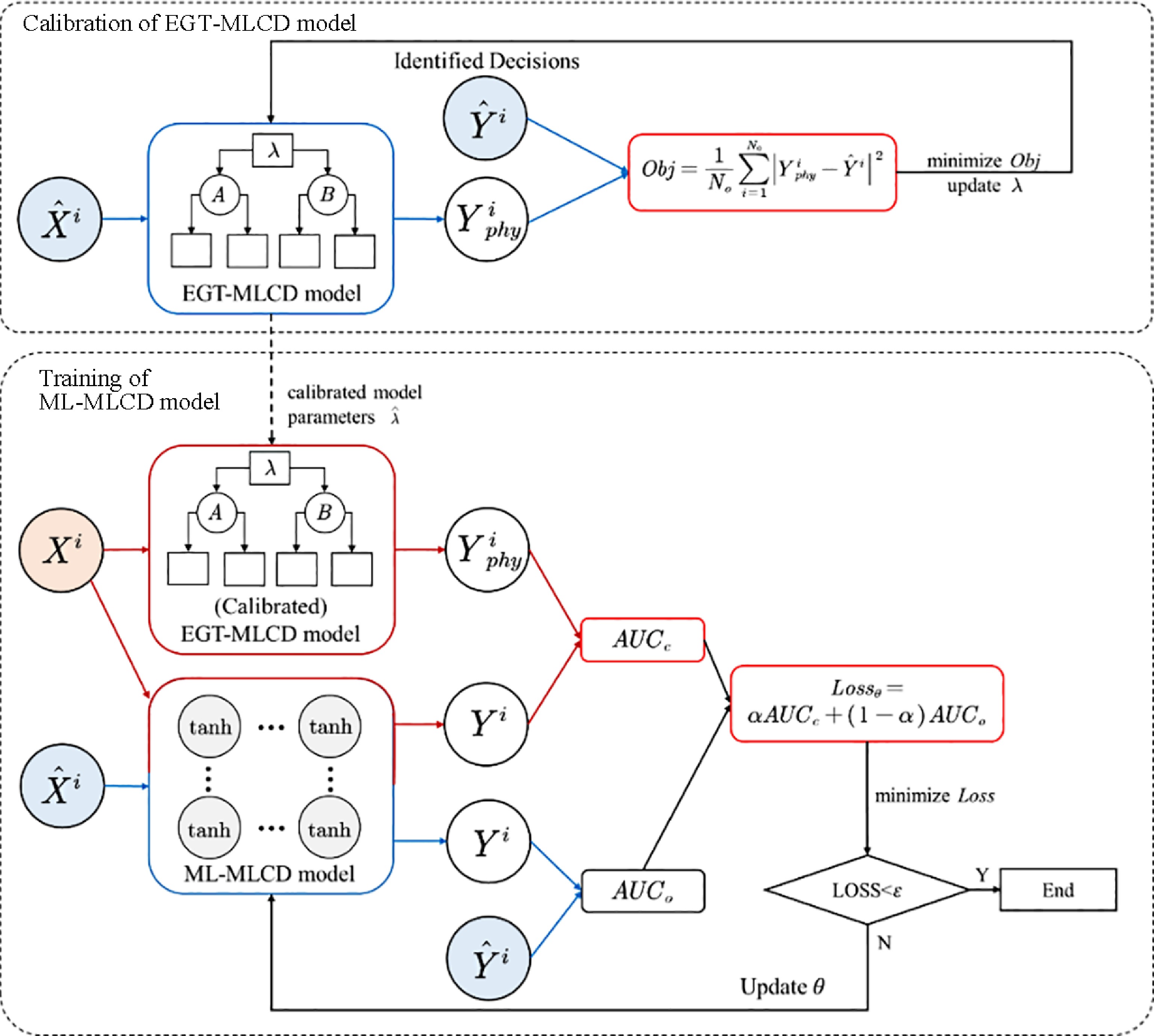
Figure 6.
Training process of EGTML.
-
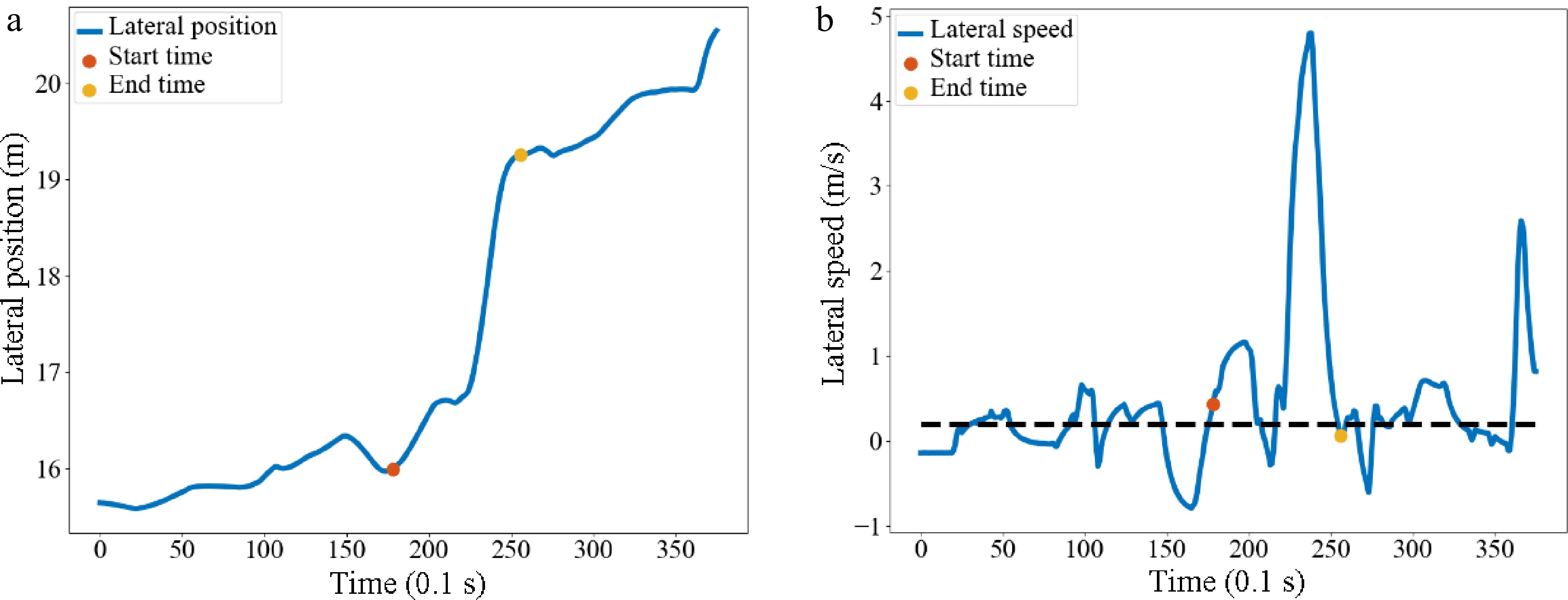
Figure 7.
Identification of the start and end time of vehicle No. 20. Diagram of (a) lateral position, (b) lateral speed.
-
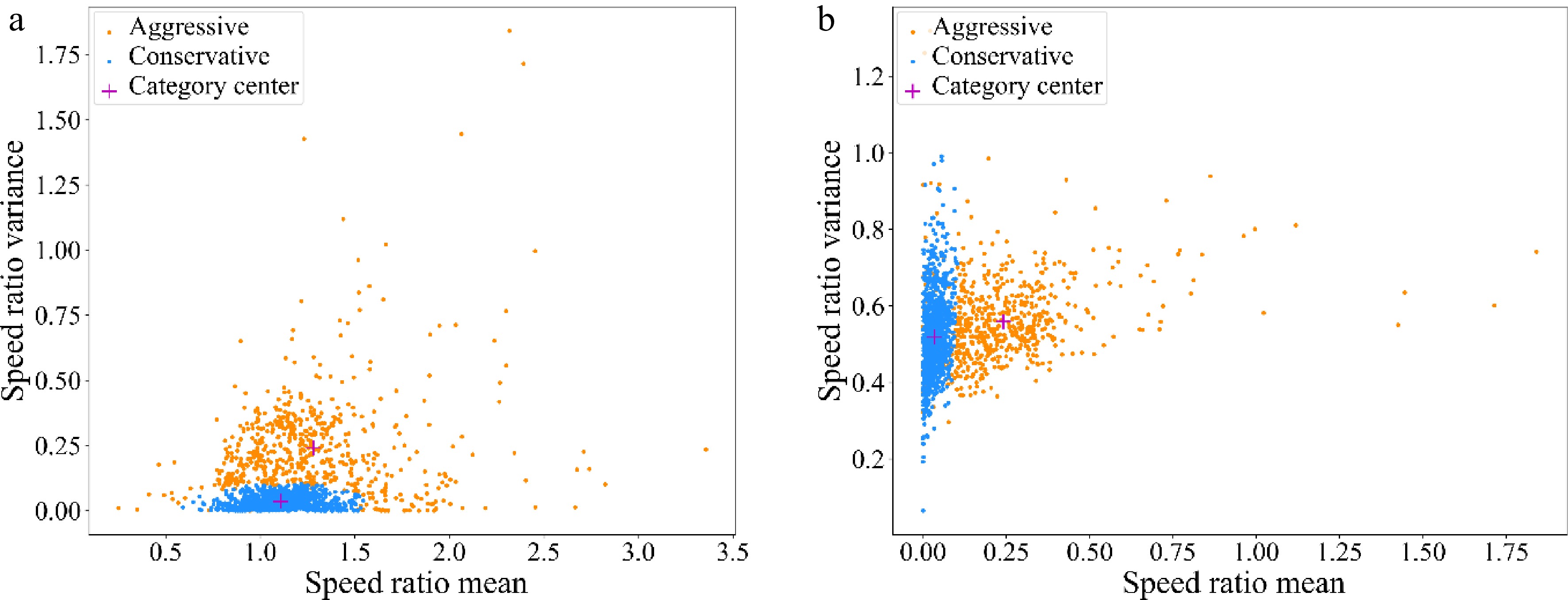
Figure 8.
Distribution of sample eigenvalues. (a) Speed ratio mean - Speed ratio variance; (b) Speed ratio variance - Acceleration mean.
-
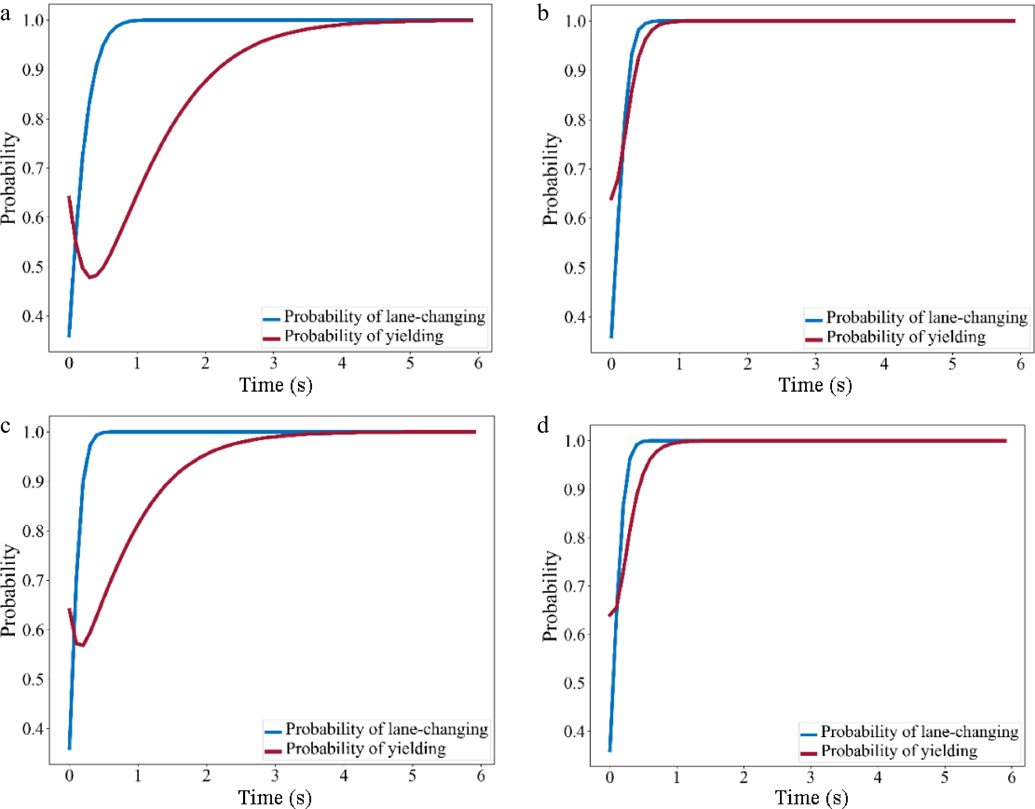
Figure 9.
Evolution diagram of probability of lane-changing and yielding. (a) Category 1 (Aggressive SV - Aggressive TB); (b) Category 2 (Aggressive SV - Conservative TB); (c) Category 3 (Conservative SV - Aggressive TB); (d) Category 4 (Conservative SV - Conservative TB).
-
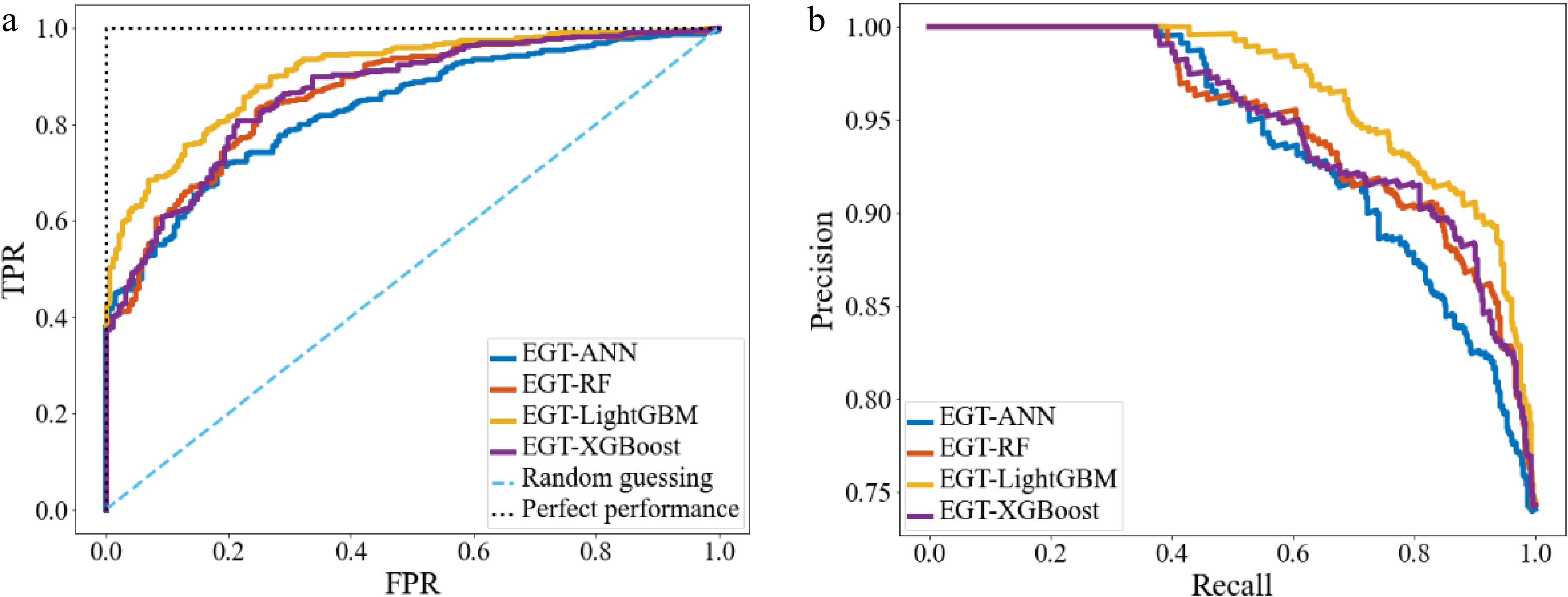
Figure 10.
The ROC curves, and PR curves of different ML models. (a) ROC curves; (b) PR curves.
-
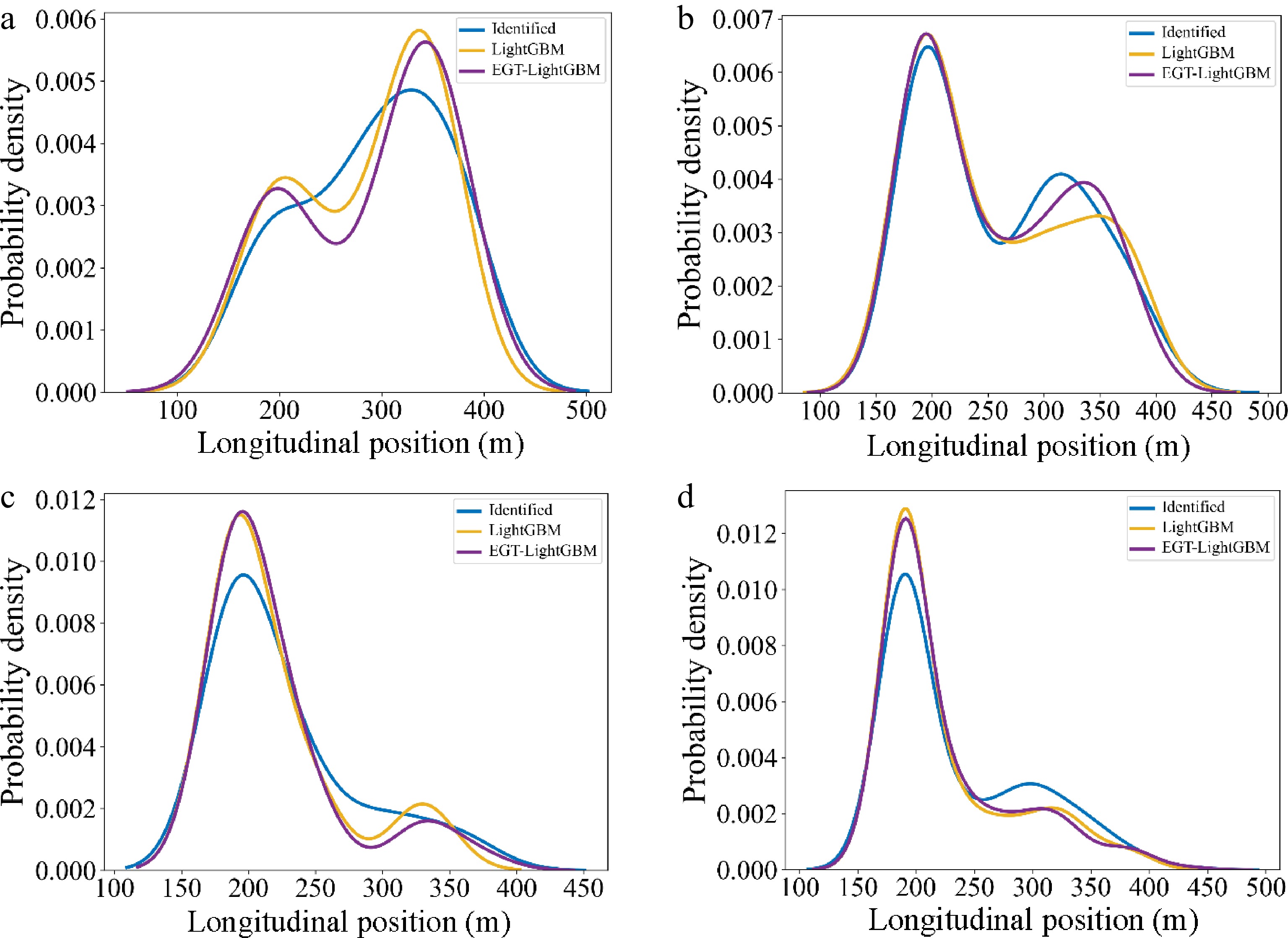
Figure 11.
Distribution of longitudinal Lane Change Decision position. (a) Category 1 (Aggressive vs Aggressive); (b) Category 2 (Aggressive vs Conservative); (c) Category 3 (Conservative vs Aggressive); (d) Category 4 (Conservative vs Conservative).
-
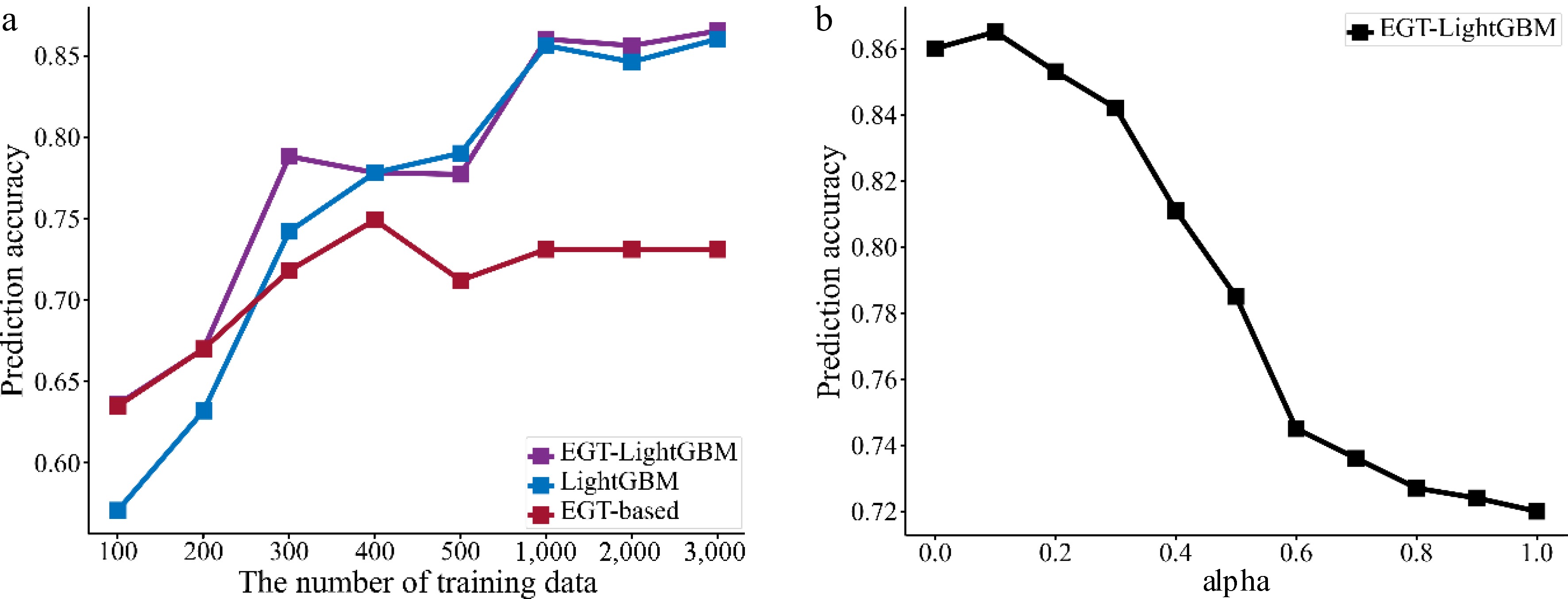
Figure 12.
The performance of EGTML. (a) Varying numbers of training data; (b) varying α.
-
Game players SV Lane change No lane change TB Yield P11 : α1TTC + β1L P21 : −β1L Q11 : α2TTC − β2Δv Q21 : −β2Δv No yield P12 : −α1TTC P22 : −β1L Q12 : β2Δv − α2TTC Q22 : β2Δv Table 1.
The payoff matrix for MLCD.
-
(x1, x2) $ F_{C V}^{\prime}\left(x^{*}\right) $ $ f_{T B}^{\prime}\left(x^{*}\right) $ Stability (0, 0) C-G F-H Determined by the payoff matrix (0,1) A-E H-F (1,0) G-C B-D (1,1) E-A D-B $\left( \dfrac{H-F}{B+H-D-F}, \dfrac{G-C}{A+G-C-E}\right) $ 0 0 Unstable solution Table 2.
Stability analysis of equilibrium solution.
-
Symbol Meaning Unit VOV, VOF, VOB, VTP, VTH The speed of the vehicle m/s AOV, AGF, ACB, ATF, ATB The acceleration of the vehicle m/s2 ΔVCF, ΔVCB, ΔVTF, ΔVTB The speed difference between vehicles m/s GCF, GCB, GTF, GTB The gap between vehicles m TTCCF, TTCCB, TTCTF, TTCTB The TTC between vehicles s L The distance of SV to the end of MLC m $ \overline{v}_{s} $ Space average speed m/s Table 3.
Features of the EGTML model.
-
Category 1 2 3 4 α1 0.98 0.99 0.96 0.97 β1 0.02 0.01 0.04 0.03 α2 0.8 0.9 0.8 0.85 β2 0.2 0.1 0.2 0.15 $ T T C _{TF}^{\min} $ 6.25 6.25 6.25 6.25 $ T T C _{TB}^{\min}$ 6.25 6.25 6.25 6.25 Table 4.
The calibration of parameters.
-
Index ANN RF LightGBM XGBoost P 0.775 0.855 0.833 0.871 R 0.963 0.931 0.944 0.933 A 0.795 0.832 0.865 0.847 Table 5.
The evaluation of different ML models.
Figures
(12)
Tables
(5)