Loading [MathJax]/jax/output/SVG/jax.js
2024 Volume 3
Article Contents
About this article
ARTICLE   Open Access    

An evolutionary game theory-based machine learning framework for predicting mandatory lane change decision

More Information
  • Mandatory lane change (MLC) is likely to cause traffic oscillations, which have a negative impact on traffic efficiency and safety. There is a rapid increase in research on mandatory lane change decision (MLCD) prediction, which can be categorized into physics-based models and machine-learning models. Both types of models have their advantages and disadvantages. To obtain a more advanced MLCD prediction method, this study proposes a hybrid architecture, which combines the Evolutionary Game Theory (EGT) based model (considering data efficient and interpretable) and the Machine Learning (ML) based model (considering high prediction accuracy) to model the mandatory lane change decision of multi-style drivers (i.e. EGTML framework). Therefore, EGT is utilized to introduce physical information, which can describe the progressive cooperative interactions between drivers and predict the decision-making of multi-style drivers. The generalization of the EGTML method is further validated using four machine learning models: ANN, RF, LightGBM, and XGBoost. The superiority of EGTML is demonstrated using real-world data (i.e., Next Generation SIMulation, NGSIM). The results of sensitivity analysis show that the EGTML model outperforms the general ML model, especially when the data is sparse.
  • Columnar cacti are plants of the Cactaceae family distributed across arid and semi-arid regions of America, with ecological, economic, and cultural value[1]. One trait that makes it possible for the columnar cactus to survive in the desert ecosystem is its thick epidermis covered by a hydrophobic cuticle, which limits water loss in dry conditions[1]. The cuticle is the external layer that covers the non-woody aerial organs of land plants. The careful control of cuticle biosynthesis could produce drought stress tolerance in relevant crop plants[2]. In fleshy fruits, the cuticle maintains adequate water content during fruit development on the plant and reduces water loss in fruit during postharvest[3]. Efforts to elucidate the molecular pathway of cuticle biosynthesis have been carried out for fleshy fruits such as tomato (Solanum lycopersicum)[4], apple (Malus domestica)[5], sweet cherry (Prunus avium)[6], mango (Mangifera indica)[7], and pear (Pyrus 'Yuluxiang')[8].

    The plant cuticle is formed by the two main layers cutin and cuticular waxes[3]. Cutin is composed mainly of oxygenated long-chain (LC) fatty acids (FA), which are synthesized by cytochrome p450 (CYP) enzymes. CYP family 86 subfamily A (CYP86A) enzymes carry out the terminal (ω) oxidation of LC-FA[9]. Then, CYP77A carries out the mid-chain oxidation to synthesize the main cutin monomers. In Arabidopsis, AtCYP77A4 and AtCYP77A6 carry out the synthesis of mid-chain epoxy and mid-chain dihydroxy LC-FA, respectively[10,11]. AtCYP77A6 is required for the cutin biosynthesis and the correct formation of floral surfaces[10]. The expression of CYP77A19 (KF410855) and CYP77A20 (KF410856) from potato (Solanum tuberosum) restored the petal cuticular impermeability in Arabidopsis null mutant cyp77a6-1, tentatively by the synthesis of cutin monomers[12]. In eggplant (Solanum torvum), the over-expression of StoCYP77A2 leads to resistance to Verticillium dahlia infection in tobacco plants[13]. Although the function of CYP77A2 in cutin biosynthesis has not yet been tested, gene expression analysis suggests that CaCYP77A2 (A0A1U8GYB0) could play a role in cutin biosynthesis during pepper fruit development[14].

    It has been hypothesized that the export of cuticle precursors is carried out by ATP binding cassette subfamily G (ABCG) transporters. ABCG11/WBC11, ABCG12, and ABCG13 are required for the load of cuticle lipids in Arabidopsis[1517], but ABCG13 function appears to be specific to the flower epidermis[18]. The overexpression of TsABCG11 (JQ389853) from Thellungiella salsugineum increases cuticle amounts and promotes tolerance to different abiotic stresses in Arabidopsis[19].

    Once exported, the cutin monomers are polymerized on the surface of epidermal cells. CD1 code for a Gly-Asp-Ser-Leu motif lipase/esterase (GDSL) from tomato required for the cutin formation through 2-mono(10,16-dihydroxyhexadecanoyl)glycerol esterification[20]. GDSL1 from tomato carries out the ester bond cross-links of cutin monomers located at the cuticle layers and is required for cuticle deposition in tomato fruits[21]. It has been shown that the transcription factor MIXTA-like reduces water loss in tomato fruits through the positive regulation of the expression of CYP77A2, ABCG11, and GDSL1[22]. Despite the relevant role of cuticles in maintaining cactus homeostasis in desert environments[1], the molecular mechanism of cuticle biosynthesis has yet to be described for cactus fruits.

    Stenocereus thurberi is a columnar cactus endemic from the Sonoran desert (Mexico), which produces an ovoid-globose fleshy fruit named sweet pitaya[23]. In its mature state, the pulp of sweet pitaya contains around 86% water with a high content of antioxidants and natural pigments such as betalains and phenolic compounds, which have nutraceutical and industrial relevance[23]. Due to the arid environment in which pitaya fruit grows, studying its molecular mechanism of cuticle biosynthesis can generate new insights into understanding species' adaptation mechanisms to arid environments. Nevertheless, sequences of transcripts from S. thurberi in public databases are scarce.

    RNA-sequencing technology (RNA-seq) allows the massive generation of almost all the transcripts from non-model plants, even if no complete assembled genome is available[24]. Recent advances in bioinformatic tools has improved our capacity to identify long non-coding RNA (lncRNA), which have been showed to play regulatory roles in relevant biological processes, such as the regulation of drought stress tolerance in plants[25], fruit development, and ripening[2629].

    In this study, RNA-seq data were obtained for the de novo assembly and characterization of the S. thurberi fruit peel transcriptome. As a first approach, three transcripts, StCYP77A, StABCG11, and StGDSL1, tentatively involved in cuticle biosynthesis, were identified and quantified during sweet pitaya fruit development. Due to no gene expression analysis having been carried out yet for S. thurberi, stably expressed constitutive genes were identified for the first time.

    Sweet pitaya fruits (S. thurberi) without physical damage were hand harvested from plants in a native conditions field located at Carbó, Sonora, México. They were collocated in a cooler containing dry ice and transported immediately to the laboratory. The superficial part of the peels (~1 mm deep) was removed carefully from the fruits using a scalpel. Peel samples from three fruits were pooled according to their tentative stage of development defined by their visual characteristics, frozen in liquid nitrogen, and pulverized to create a single biological replicate. Four samples belonging to four different plants were analyzed. All fruits harvested were close to the ripening stage. Samples named M1 and M2 were turning from green to ripe [~35−40 Days After Flowering (DAF)], whereas samples M3 and M4 were turning from ripe to overripe (~40−45 DAF).

    Total RNA was isolated from the peels through the Hot Borate method[30]. The concentration and purity of RNA were determined in a spectrophotometer Nanodrop 2000 (Thermo Fisher) by measuring the 260/280 and 260/230 absorbance ratios. RNA integrity was evaluated through electrophoresis in agarose gel 1% and a Bioanalyzer 2100 (Agilent). Pure RNA was sequenced in the paired-end mode in an Illumina NextSeq 500 platform at the University of Arizona Genetics Core Facility. Four RNA-seq libraries, each of them from each sample, were obtained, which include a total of 288,199,704 short reads with a length of 150 base pairs (bp). The resulting sequence data can be accessed at the Sequence Read Archive (SRA) repository of the NCBI through the BioProject ID PRJNA1030439. Libraries are named corresponding to the names of samples M1, M2, M3, and M4.

    FastQC software (www.bioinformatics.babraham.ac.uk/projects/fastqc) was used for short reads quality analysis. Short reads with poor quality were trimmed or eliminated by Trimmomatic (www.usadellab.org/cms/?page=trimmomatic) with a trailing and leading of 25, a sliding window of 4:25, and a minimum read length of 80 bp. A total of 243,194,888 reads with at least a 25 quality score on the Phred scale were used to carry out the de novo assembly by Trinity (https://github.com/trinityrnaseq/trinityrnaseq/wiki) with the following parameters: minimal k-mer coverage of 1, normalization of 50, and minimal transcript length of 200 bp.

    Removal of contaminating sequences and ribosomal RNA (rRNA) was carried out through SeqClean. To remove redundancy, transcripts with equal or more than 90% of identity were merged through CD-hit (www.bioinformatics.org/cd-hit/). Alignment and quantification in terms of transcripts per million (TPM) were carried out through Bowtie (https://bowtie-bio.sourceforge.net/index.shtml) and RSEM (https://github.com/deweylab/RSEM), respectively. Transcripts showing a low expression (TPM < 0.01) were discarded. Assembly quality was evaluated by calculating the parameters N50 value, mean transcript length, TransRate score, and completeness. The statistics of the transcriptome were determined by TrinityStats and TransRate (https://hibberdlab.com/transrate/). The transcriptome completeness was determined through a BLASTn alignment (E value < 1 × 10⁻³) by BUSCO (https://busco.ezlab.org/) against the database of conserved orthologous genes from Embryophyte.

    To predict the proteins tentatively coded in the S. thurberi transcriptome, the best homology match of the assembled transcripts was found by alignment to the Swiss-Prot, RefSeq, nr-NCBI, PlantTFDB, iTAK, TAIR, and ITAG databases using the BLAST algorithm with an E value threshold of 1 × 10⁻¹⁰ for the nr-NCBI database and of 1 × 10⁻⁵ for the others[3134]. An additional alignment was carried out to the protein databases of commercial fruits Persea americana, Prunus persica, Fragaria vesca, Citrus cinensis, and Vitis vinifera to proteins of the cactus Opuntia streptacantha, and the transcriptomes of the cactus Hylocereus polyrhizus, Pachycereus pringlei, and Selenicereus undatus. The list of all databases and the database websites of commercial fruits and cactus are provided in Supplementary Tables S1 & S2. The open reading frame (ORF) of the transcripts and the protein sequences tentative coded from the sweet pitaya transcriptome was predicted by TransDecoder (https://github.com/TransDecoder/TransDecoder/wiki), considering a minimal ORF length of 75 amino acids (aa). The search for protein domains was carried out by the InterPro database (www.ebi.ac.uk/interpro). Functional categorization was carried out by Blast2GO based on GO terms and KEGG metabolic pathways[35].

    LncRNA were identified based on the methods reported in previous studies[25,29,36]. Transcripts without homology to any protein from Swiss-Prot, RefSeq, nr-NCBI, PlantTFDB, iTAK, TAIR, ITAG, P. americana, P. persica, F. vesca, C. cinensis, V. vinifera, and O. streptacantha databases, without a predicted ORF longer than 75 aa, and without protein domains in the InterPro database were selected to identify tentative lncRNA.

    Transcripts coding for signal peptide or transmembrane helices were identified by SignalP (https://services.healthtech.dtu.dk/services/SignalP-6.0/) and TMHMM (https://services.healthtech.dtu.dk/services/TMHMM-2.0/), respectively, and discarded. Further, transcripts corresponding to other non-coding RNAs (ribosomal RNA and transfer RNA) were identified through Infernal by using the Rfam database[37] and discarded. The remaining transcripts were analyzed by CPC[38], and CPC2[39] to calculate their coding potential. Transcripts with a coding potential score lower than −1 for CPC and a coding probability lower than 0.1 for CPC2 were considered lncRNA. To characterize the identified lncRNA, the length and abundance of coding and lncRNA were calculated. Bowtie and RSEM were used to align and quantify raw counts, respectively. The edgeR package[40] was used to normalize raw count data in terms of counts per million (CPM) for both coding and lncRNA.

    To obtain the transcript's expression, the aligning of short reads and quantifying of transcripts were carried out through Bowtie and RSEM software, respectively. A differential expression analysis was carried out between the four libraries by edgeR package in R Studio. Only the transcripts with a count equal to or higher than 0.5 in at least one sample were retained for the analysis. Transcripts with log2 Fold Change (log2FC) between +1 and −1 and with a False Discovery Rate (FDR) lower than 0.05 were taken as not differentially expressed (NDE).

    For the identification of the tentative reference genes two strategies were carried out as described below: i) The NDE transcripts were aligned by BLASTn (E value < 1 × 10⁻⁵) to 43 constitutive genes previously reported in fruits from the cactus H. polyrhizus, S. monacanthus, and S. undatus[4143] to identify possible homologous constitutive genes in S. thurberi. Then, the homologous transcripts with the minimal coefficient of variation (CV) were selected; ii) For all the NDE transcripts, the percentile 95 value of the mean CPM and the percentile 5 value of the CV were used as filters to recover the most stably expressed transcripts, based on previous studies[44]. Finally, transcripts to be tested by quantitative reverse transcription polymerase chain reaction (qRT-PCR) were selected based on their homology and tentative biological function.

    The fruit harvesting was carried out as described above. Sweet pitaya fruit takes about 43 d to ripen, therefore, open flowers were tagged, and fruits with 10, 20, 30, 35, and 40 DAF were collected to cover the pitaya fruit development process (Supplementary Fig. S1). The superficial part of the peels (~1 mm deep) was removed carefully from the fruits using a scalpel. Peel samples from three fruits were pooled according to their stage of development defined by their DAF, frozen in liquid nitrogen, and pulverized to create a single biological replicate. One biological replicate consisted of peels from three fruits belonging to the same plant. Two to three biological replicates were evaluated for each developmental stage. Two technical replicates were analyzed for each biological replicate. RNA extraction, quantification, RNA purity, and RNA integrity analysis were carried out as described above.

    cDNA was synthesized from 100 ng of RNA by QuantiTect Reverse Transcription Kit (QIAGEN). Primers were designed using the PrimerQuest™, UNAFold, and OligoAnalyzer™ tools from Integrated DNA Technologies (www.idtdna.com/pages) and following the method proposed by Thornton & Basu[45]. Transcripts quantification was carried out in a QIAquant 96 5 plex according to the PowerUp™ SYBR™ Green Master Mix protocol (Applied Biosystems), with a first denaturation step for 2 min at 95 °C, followed by 40 cycles of denaturation step at 95 °C for 15 s, annealing and extension steps for 30 s at 60 °C.

    The Cycle threshold (Ct) values obtained from the qRT-PCR were analyzed through the algorithms BestKeeper, geNorm, NormFinder, and the delta Ct method[46]. RefFinder (www.ciidirsinaloa.com.mx/RefFinder-master/) was used to integrate the stability results and to find the most stable expressed transcripts in sweet pitaya fruit peel during development. The pairwise variation value (Vn/Vn + 1) was calculated through the geNorm algorithm in R Studio software[47].

    An alignment of 17 reported cuticle biosynthesis genes from model plants were carried out by BLASTx against the predicted proteins from sweet pitaya. Two additional alignments of 17 charaterized cuticle biosynthesis proteins from model plants against the transcripts and predicted proteins of sweet pitaya were carried out by tBLASTn and BLASTp, respectively. An E value threshold of 1 × 10⁻⁵ was used, and the unique best hits were recovered for all three alignments. The sequences of the 17 characterized cuticle biosynthesis genes and proteins from model plants are showed in Supplementary Table S3. The specific parameters and the unique best hits for all the alignments carried out are shown in Supplementary Tables S4S8.

    Cuticle biosynthesis-related transcripts tentatively coding for a cytochrome p450 family 77 subfamily A (CYP77A), a Gly-Asp-Ser-Leu motif lipase/esterase 1 (GDSL1), and an ATP binding cassette transporter subfamily G member 11 (ABCG11) were identified by best bi-directional hit according to the functional annotation described above. Protein-conserved domains, signal peptide, and transmembrane helix were predicted through InterProScan, SignalP 6.0, and TMHMM, respectively. Alignment of the protein sequences to tentative orthologous of other plant species was carried out by the MUSCLE algorithm[48]. A neighbor-joining (NJ) phylogenetic tree with a bootstrap of 1,000 replications was constructed by MEGA11[49].

    Fruit sampling, primer design, RNA extraction, cDNA synthesis, and transcript quantification were performed as described above. Relative expression was calculated according to the 2−ΔΔCᴛ method[50]. The sample corresponding to 10 DAF was used as the calibrator. The transcripts StEF1a, StTUA, StUBQ3, and StEF1a + StTUA were used as normalizer genes.

    Normality was assessed according to the Shapiro-Wilk test. Significant differences in the expression of the cuticle biosynthesis-related transcripts between fruit developmental stages were determined by one-way ANOVA based on a completely randomized sampling design and a Tukey honestly significant difference (HSD) test, considering a p-value < 0.05 as significant. Statistical analysis was carried out through the stats package in R Studio.

    RNA was extracted from the peels of ripe sweet pitaya fruits (S. thurberi) from plants located in the Sonoran Desert, Mexico. Four cDNA libraries were sequenced in an Illumina NextSeq 500 platform at the University of Arizona Genetics Core Facility. A total of 288,199,704 reads with 150 base pairs (bp) in length were sequenced in paired-end mode. After trimming, 243,194,888 (84.38%) cleaned short reads with at least 29 mean quality scores per read in the Phred scale and between 80 to 150 bp in length were obtained to carry out the assembly. After removing contaminating sequences, redundancy, and low-expressed transcripts, the assembly included 174,449 transcripts with an N50 value of 2,110 bp. Table 1 shows the different quality variables of the S. thurberi fruit peel transcriptome. BUSCO score showed that 85.4% are completed transcripts, although out of these, 37.2% were found to be duplicated. The resulting sequence data can be accessed at the SRA repository of the NCBI through the BioProject ID PRJNA1030439.

    Table 1.  Quality metrics of the Stenocereus thurberi fruit peel transcriptome.
    Metric Data
    Total transcripts 174,449
    N50 2,110
    Smallest transcript length (bp) 200
    Largest transcript length (bp) 19,114
    Mean transcript length (bp) 1,198.69
    GC (%) 41.33
    Total assembled bases 209,110,524
    TransRate score 0.05
    BUSCO score (%) C: 85.38 (S:48.22, D:37.16),
    F: 10.69, M: 3.93.
    Values were calculated through the TrinityStats function of Trinity and TransRate software. Completeness analysis was carried out through BUSCO by aligning the transcriptome to the Embryophyte database through BLAST with an E value threshold of 1 × 10⁻³. Complete (C), single (S), duplicated (D), fragmented (F), missing (M).
     | Show Table
    DownLoad: CSV

    A summary of the homology search in the main public protein database for the S. thurberi transcriptome is shown in Supplementary Table S1. From these databases, the higher homologous transcripts were found in RefSeq with 93,993 (53.87 %). Based on the E value distribution, for 41,685 (44%) and 68,853 (49%) of the hits, it was found a strong homology (E value lower than 1 × 10−50) to proteins in the Swiss-Prot and RefSeq databases, respectively (Supplementary Fig. S2a & b). On the other hand, 56,539 (52.34%) and 99,599 (71.11%) of the matches showed a percentage of identity higher than 60% in the Swiss-Prot and RefSeq databases, respectively (Supplementary Fig. S2c & d).

    Figure 1 shows the homology between transcripts from S. thurberi and proteins of commercial fruits, as well as proteins and transcripts of cacti. Transcripts from S. thurberi homologous to proteins from fruits of commercial interest avocado (P. americana), peach (P. persica), strawberry (F. vesca), orange (C. sinensis), and grapefruit (V. vinifera) ranged from 77,285 (44.30%) to 85,421 (48.96%), with 70,802 transcripts homologous to all the five fruit protein databases (Fig. 1a).

    Transcripts homologous to transcripts or proteins from the cactus dragon fruit (H. polyrhizus), prickly pear cactus (O. streptacantha), Mexican giant cardon (P. pringlei), and pitahaya (S. undatus) ranged from 76,238 (43.70%) to 114,933 (65.88%), with 64,009 transcripts homologous to all the four cactus databases (Fig. 1b). Further, out of the total of transcripts, 44,040 transcripts (25.25%) showed homology only to sequences from cactus, but not for model plants Arabidopsis, tomato, or the commercial fruits included in this study (Fig. 1c).

    Figure 1.  Venn diagram of the homology search results against model plants databases, commercial fruits, and cactus. The number in the diagram corresponds to the number of transcripts from S. thurberi homologous to sequences from that plant species. (a) Homologous to sequences from Fragaria vesca (Fa), Persea americana (Pa), Prunus persica (Pp), Vitis vinifera (Vv), and Citrus sinensis (Cs). (b) Homologous to sequences from Opuntia streptacantha (Of), Selenicereus undatus (Su), Hylocereus polyrhizus (Hp), and Pachycereus pringlei (Pap). (c) Homologous to sequences from Solanum lycopersicum (Sl), Arabidopsis thaliana (At), from the commercial fruits (Fa, Pa, Pp, Vv, and Cs), or the cactus included in this study (Of, Su, Hp, and Pap). Homologous searching was carried out by BLAST alignment (E value < 1 × 10⁻⁵). The Venn diagrams were drawn by ggVennDiagram in R Studio.

    A total of 45,970 (26.35%), 58,704 (33.65%), and 48,186 (27.65%) transcripts showed homology to transcription factors, transcriptional regulators, and protein kinases in the PlantTFDB, iTAK-TR, and iTAK-PK databases, respectively (Supplementary Tables S1, S9S11). For the PlantTFDB, the homologous transcripts belong to 57 transcriptional factors (TF) families (Fig. 2 & Supplementary Table S9), from which, the most frequent were the basic-helix-loop-helix (bHLH), myeloblastosis-related (MYB-related), NAM, ATAF, and CUC (NAC), ethylene responsive factor (ERF), and the WRKY domain families (WRKY) (Fig. 2).

    Figure 2.  Transcription factor (TF) families distribution of S. thurberi fruit peel transcriptome. The X-axis indicates the number of transcripts with hits to each TF family. Alignment to the PlantTFDB database by BLASTx was carried out with an E value threshold of 1 × 10⁻⁵. The bar graph was drawn by ggplot2 in R Studio.

    Based on the homology found and the functional domain searches, gene ontology terms (GO) were assigned to 68,559 transcripts (Supplementary Table S12). Figure 3 shows the top 20 GO terms assigned to the S. thurberi transcriptome, corresponding to the Biological Processes (BP) and Molecular Function (MF) categories. For BP, organic substance metabolic processes, primary metabolic processes, and cellular metabolic processes showed a higher number of transcripts (Supplementary Table S13). Further, for MF, organic cyclic compound binding, heterocyclic compound binding, and ion binding were the processes with the higher number of transcripts. S. thurberi transcripts were classified into 142 metabolic pathways from the KEGG database (Supplementary Table S14). The pathways with the higher number of transcripts recorded were pyruvate metabolism, glycerophospholipid metabolism, glycolysis/gluconeogenesis, and citrate cycle. Further, among the top 20 KEEG pathways, the cutin, suberin, and wax biosynthesis include more than 30 transcripts (Fig. 4).

    Figure 3.  Top 20 Gene Ontology (GO) terms assigned to the S. thurberi fruit peel transcriptome. Bars indicate the number of transcripts assigned to each GO term. Assignment of GO terms was carried out by Blast2GO with default parameters. BP and MF mean Biological Processes and Molecular Functions GO categories, respectively. The graph was drawn by ggplot2 in R Studio.
    Figure 4.  Top 20 KEGG metabolic pathways distribution in the S. thurberi fruit peel transcriptome. Bars indicate the number of transcripts assigned to each KEGG pathway. Assignment of KEGG pathways was carried out in the Blast2GO suite. The bar graph was drawn by ggplot2 in R Studio.

    Out of the total of transcripts, 43,391 (24.87%) were classified as lncRNA (Supplementary Tables S15 & S16). Figure 5 shows a comparison of the length (Fig. 5a) and expression (Fig. 5b) of lncRNA and coding RNA. Both length and expression values were higher in coding RNA than in lncRNA. In general, coding RNA ranged from 201 to 18,629 bp with a mean length of 1,507.18, whereas lncRNA ranged from 200 to 5,198 bp with a mean length of 481.51 (Fig. 5a). The higher expression values recorded from coding RNA and lncRNA were 12.83 and 9.45 log2(CPM), respectively (Fig. 5b).

    Figure 5.  Comparison of coding RNA and long non-coding RNA (lncRNA) from S. thurberi transcriptome. (a) Box plot of transcript length distribution. The Y-axis indicates the length of each transcript in base pairs. (b) Box plot of expression levels. The Y-axis indicates the log2 of the count per million of reads (log2(CPM)) recorded for each transcript. Expression levels were calculated by the edgeR package in R studio. (a), (b) The lines inside the boxes indicate the median. The higher and lower box limits represent the 75th and 25th percentiles, respectively. The box plots were drawn by ggplot2 in R Studio.

    To identify the transcripts without significant changes in expression between the four RNA-seq libraries, a differential expression analysis was carried out. Of the total of transcripts, 4,980 were not differentially expressed (NDE) at least in one paired comparison between the libraries (Supplementary Tables S17S20). Mean counts per million of reads (CPM) and coefficient of variation (CV)[44] were calculated for these NDE transcripts. Transcripts with a CV value lower than 0.113, corresponding with the percentile 5 of the CV, and a mean CPM higher than 1,138.06, corresponding with the percentile 95 of the mean CPM were used as filters to identify the most stably expressed transcripts (Supplementary Table S21). Based on its homology and its tentative biological function, five transcripts were selected to be tested as tentative reference genes. Besides, three NDE transcripts homologous to previously identified stable expressed reference genes in other species of cactus fruit[4143] were selected (Supplementary Table S22). Homology metrics for the eight tentative reference genes selected are shown in Supplementary Table S23. The primer sequences used to amplify the transcripts by qRT-PCR and their nucleotide sequence are shown in Supplementary Tables S24 & S25, respectively.

    The amplification specificity of the eight candidate reference genes determined by melting curves analysis is shown in Supplementary Fig. S3. For the eight tentative reference transcripts selected, the cycle threshold (Ct) values were recorded during sweet pitaya fruit development by qRT-PCR (Supplementary Table S26). The Ct values obtained ranged from 16.85 to 30.26 (Fig. 6a). Plastidic ATP/ADP-transporter (StTLC1) showed the highest Ct values with a mean of 27.34 (Supplementary Table S26). Polyubiquitin 3 (StUBQ3) showed the lowest Ct values in all five sweet pitaya fruit developmental stages (Fig. 6a).

    Figure 6.  Expression stability analysis of tentative reference genes. (a) Box plot of cycle threshold (Ct) distribution of candidate reference genes during sweet pitaya fruit development (10, 20, 30, 35, and 40 d after flowering). The black line inside the box indicates the median. The higher and lower box limits represent the 75th and 25th percentiles, respectively. (b) Bar chart of the geometric mean (geomean) of ranking values calculated by RefFinder for each tentative reference gene (X-axis). The lowest values indicate the best reference genes. (c) Bar chart of the pairwise variation analysis and determination of the optimal number of reference genes by the geNorm algorithm. A pairwise variation value lower than 0.15 indicates that the use of Vn/Vn + 1 reference genes is reliable for the accurate normalization of qRT-PCR data. The Ct data used in the analysis were calculated by qRT-PCR in a QIAquant 96 5 plex (QIAGEN) according to the manufacturer's protocol. The box plot and the bar graphs were drawn by ggplot2 and Excel programs, respectively. Abbreviations: Actin 7 (StACT7), alpha-tubulin (StTUA), elongation factor 1-alpha (StEF1a), COP1-interactive protein 1 (StCIP1), plasma membrane ATPase 4 (StPMA4), BEL1-like homeodomain protein 1 (StBLH1), polyubiquitin 3 (StUBQ3), and plastidic ATP/ADP-transporter (StTLC1).

    The best stability values calculated by NormFinder were 0.45, 0.51, 0.97, and 0.99, corresponding to the transcripts elongation factor 1-alpha (StEF1a), alpha-tubulin (StTUA), plastidic ATP/ADP-transporter (StTLC1), and actin 7 (StACT7), respectively (Supplementary Table S27). For BestKeeper, the most stable expressed transcripts were StUBQ3, StTUA, and StEF1a, with values of 0.72, 0.75, and 0.87, respectively. In the case of the delta Ct method[51], the transcripts StEF1a, StTUA, and StTLC1 showed the best stability.

    According to geNorm analysis, the most stable expressed transcripts were StTUA, StEF1a, StUBQ3, and StACT7, with values of 0.74, 0.74, 0.82, and 0.96, respectively. All the pairwise variation values (Vn/Vn + 1) were lower than 0.15, ranging from 0.019 for V2/V3 to 0.01 for V6/V7 (Fig. 6c). The V value of 0.019 obtained for V2/V3 indicates that the use of the best two reference genes StTUA and StEF1a is reliable enough for the accurate normalization of qRT-PCR data, therefore no third reference gene is required[47]. Except for BestKeeper analysis, StEF1a and StTUA were the most stable transcripts for all of the methods carried out in this study (Supplementary Table S27). The comprehensive ranking analysis indicates that StEF1a, followed by StTUA and StUBQ3, are the most stable expressed genes and are stable enough to be used as reference genes in qRT-PCR analysis during sweet pitaya fruit development (Fig. 6b).

    Three cuticle biosynthesis-related transcripts TRINITY_DN17030_c0_g1_i2, TRINITY_DN15394_c0_g1_i1, and TRINITY_DN23528_c1_g1_i1 tentatively coding for the enzymes cytochrome p450 family 77 subfamily A (CYP77A), Gly-Asp-Ser-Leu motif lipase/esterase 1 (GDSL1), and an ATP binding cassette transporter subfamily G member 11 (ABCG11/WBC11), respectively, were identified and quantified. The nucleotide sequence and predicted amino acid sequences of the three transcripts are shown in Supplementary File 1. The best homology match for StCYP77A (TRINITY_DN17030_c0_g1_i2) was for AtCYP77A4 (AT5G04660) from Arabidopsis and SmCYP77A2 (P37124) from eggplant (Solanum melongena) in the TAIR and Swiss-Prot databases, respectively (Supplementary Table S23).

    TransDecoder, InterPro, and TMHMM analysis showed that StCYP77A codes a polypeptide of 518 amino acids (aa) in length that comprises a cytochrome P450 E-class domain (IPR002401) and a transmembrane region (residues 10 to 32). The phylogenetic tree constructed showed that StCYP77A is grouped in a cluster with all the CYP77A2 proteins included in this analysis, being closer to CYP77A2 (XP_010694692) from B. vulgaris and Cgig2_012892 (KAJ8441854) from Carnegiea gigantean (Supplementary Fig. S4).

    StGDSL1 (TRINITY_DN15394_c0_g1_i1) alignment showed that it is homologous to a GDSL esterase/lipase from Arabidopsis (Q9LU14) and tomato (Solyc03g121180) (Supplementary Table S23). TransDecoder, InterPro, and SignalP analysis showed that StGDSL1 codes a polypeptide of 354 aa in length that comprises a GDSL lipase/esterase domain IPR001087 and a signal peptide with a cleavage site between position 25 and 26 (Supplementary Fig. S5).

    Supplementary Figure S6 shows the analysis carried out on the predicted amino acid sequence of StABCG11 (TRINITY_DN23528_c1_g1_i1). The phylogenetic tree constructed shows three clades corresponding to the ABCG13, ABCG12, and ABCG11 protein classes with bootstrap support ranging from 40% to 100% (Supplementary Fig. S6a). StABCG11 is grouped with all the ABCG11 transporters included in this study in a well-separated clade, being closely related to its tentative ortholog from C. gigantean Cgig2_004465 (KAJ8441854). InterPro and TMHMM results showed that the StABCG11 sequence contains an ABC-2 type transporter transmembrane domain (IPR013525; PF01061.27) with six transmembrane helices (Supplementary Fig. S6b).

    The predicted protein sequence of StABCG11 is 710 aa in length, holding the ATP binding domain (IPR003439; PF00005.30) and the P-loop containing nucleoside triphosphate hydrolase domain (IPR043926; PF19055.3) of the ABC transporters of the G family. Multiple sequence alignment shows that the Walker A and B motif sequence and the ABC signature[15] are conserved between the ABCG11 transporters from Arabidopsis, tomato, S. thurberi, and C. gigantean (Supplementary Fig. S6c).

    According to the results of the expression stability analysis (Fig. 6), four normalization strategies were tested to quantify the three cuticle biosynthesis-related transcripts during sweet pitaya fruit development. The four strategies consist of normalizing by StEF1a, StTUA, StUBQ3, or StEF1a+StTUA. Primer sequences used to quantify the transcripts StCYP77A (TRINITY_DN17030_c0_g1_i2), StGDSL1 (TRINITY_DN15394_c0_g1_i1), and StABCG11 (TRINITY_DN23528_c1_g1_i1) by qRT-PCR during sweet pitaya fruit development are shown in Supplementary Table S24.

    The three cuticle biosynthesis-related transcripts showed differences in expression during sweet pitaya fruit development (Supplementary Table S28). The same expression pattern was recorded for the three cuticle biosynthesis transcripts when normalization was carried out by StEF1a, StTUA, StUBQ3, or StEF1a + StTUA (Fig. 7). A higher expression of StCYP77A and StGDSL1 are shown at the 10 and 20 DAF, showing a decrease at 30, 35, and 40 DAF. StABCG11 showed a similar behavior, with a higher expression at 10 and 20 DAF and a reduction at 30 and 35 DAF. Nevertheless, unlike StCYP77A and StGDSL1, a significant increase at 40 DAF, reaching the same expression as compared with 10 DAF, is shown for StABCG11 (Fig. 7).

    Figure 7.  Expression analysis of cuticle biosynthesis-related transcripts StCYP77A, StGDSL1, and StABCG11 during sweet pitaya (Stenocereus thurberi) fruit development. Relative expression was calculated through the 2−ΔΔCᴛ method using elongation factor 1-alpha (StEF1a), alpha-tubulin (StTUA), polyubiquitin 3 (StUBQ3), or StEF1a + StTUA as normalizing genes at 10, 20, 30, 35, and 40 d after flowering (DAF). The Y-axis and error bars represent the mean of the relative expression ± standard error (n = 4−6) for each developmental stage in DAF. The Ct data for the analysis was recorded by qRT-PCR in a QIAquant 96 5 plex (QIAGEN) according to the manufacturer's protocol. The graph line was drawn by ggplot2 in R Studio. Abbreviations: cytochrome p450 family 77 subfamily A (StCYP77A), Gly-Asp-Ser-Leu motif lipase/esterase 1 (StGDSL1), and ATP binding cassette transporter subfamily G member 11 (StABCG11).

    Characteristics of a well-assembled transcriptome include an N50 value closer to 2,000 bp, a high percentage of conserved transcripts completely assembled (> 80%), and a high proportion of reads mapping back to the assembled transcripts[52]. In the present study, the first collection of 174,449 transcripts from S. thurberi fruit peel are reported. The generated transcriptome showed an N50 value of 2,110 bp, a TransRate score of 0.05, and a GC percentage of 41.33 (Table 1), similar to that reported for other de novo plant transcriptome assemblies[53]. According to BUSCO, 85.4% of the orthologous genes from the Embryophyta databases completely matched the S. thurberi transcriptome, and only 3.9% were missing (Table 1). These results show that the S. thurberi transcriptome generated is not fragmented, and it is helpful in predicting the sequence of almost all the transcripts expressed in sweet pitaya fruit peel[24].

    The percentage of transcripts homologous found, E values, and identity distribution (Supplementary Tables S1 & S2; Supplementary Fig. S2) were similar to that reported in the de novo transcriptome assembly for non-model plants and other cactus fruits[4143,54] and further suggests that the transcriptome assembled of S. thurberi peel is robust[52]. Of the total of transcripts, 70,802 were common to all the five commercial fruit protein databases included in this study, which is helpful for the search for conserved orthologous involved in fruit development and ripening (Fig. 2a). A total of 34,513 transcripts (20%) show homology only to sequences in the cactus's databases, but not in the others (Supplementary Tables S1 & S2; Fig. 1c). This could suggest that a significant conservation of sequences among plants of the Cactaceae family exists which most likely are to have a function in this species adaptation to desert ecosystems.

    To infer the biological functionality represented by the S. thurberi fruit peel transcriptome, gene ontology (GO) terms and KEGG pathways were assigned. Of the main metabolic pathways assigned, 'glycerolipid metabolism' and 'cutin, suberine, and wax biosynthesis' suggests an active cuticle biosynthesis in pitaya fruit peel (Fig. 4). In agreement with the above, the main GO terms assigned for the molecular function (MF) category were 'organic cyclic compound binding', 'transmembrane transporter activity', and 'lipid binding' (Fig. 3). For the biological processes (BP) category, the critical GO terms for the present research are 'cellular response to stimulus', 'response to stress', 'anatomical structure development', and 'transmembrane transport', which could suggest the active development of the fruit epidermis and cuticle biosynthesis for protection to stress.

    The most frequent transcription factors (TF) families found in S. thurberi transcriptome were NAC, WRKY, bHLH, ERF, and MYB-related (Fig. 2), which had been reported to play a function in the tolerance to abiotic stress in plants[55,56]. Although the role of NAC, WRKY, bHLH, ERF, and MYB TF in improving drought tolerance in relevant crop plants has been widely documented[57,58], their contribution to the adaptation of cactus to arid ecosystems has not yet been elucidated and further experimental pieces of evidence are needed.

    It has been reported that the heterologous expression of ERF TF from Medicago truncatula induces drought tolerance and cuticle wax biosynthesis in Arabidopsis leaf[59]. In tomato fruits, the gene SlMIXTA-like which encodes a MYB transcription factor avoids water loss through the positive regulation of genes related to the biosynthesis and transport of cuticle compounds[22]. Despite the relevant role of cuticles in maintaining cactus physiology in desert environments, experimental evidence showing the role of the different TF-inducing cuticle biosynthesis has yet to be reported for cactus fruits.

    Out of the transcripts, 43,391 were classified as lncRNA (Supplementary Tables S15 & S16). This is the first report of lncRNA identification for the species S. thurberi. In fruits, 3,679 lncRNA has been identified from tomato[26], 3,330 from peach (P. persica)[29], 3,857 from melon (Cucumis melo)[28], 2,505 from hot pepper (Capsicum annuum)[27], and 3,194 from pomegranate (Punica granatum)[36]. Despite the stringent criteria to classify the lncRNA of sweet pitaya fruit (S. thurberi), a higher number of lncRNAs are shown when compared with previous reports. This finding is most likely due to the higher level of redundancy found during the transcriptome analysis. To reduce this redundancy, further efforts to achieve the complete genome assembly of S. thurberi are needed.

    Previous studies showed that lncRNA is shorter and has lower expression levels than coding RNA[6062]. In agreement with those findings, both the length and expression values of lncRNA from S. thurberi were lower than coding RNA (Fig. 5). It has been suggested that lncRNA could be involved in the biosynthesis of cuticle components in cabbage[61] and pomegranate[36] and that they could be involved in the tolerance to water deficit through the regulation of cuticle biosynthesis in wild banana[60]. Nevertheless, the molecular mechanism by which lncRNA may regulate the cuticle biosynthesis in S. thurberi fruits has not yet been elucidated.

    A relatively constant level of expression characterizes housekeeping genes because they are involved in essential cellular functions. These genes are not induced under specific conditions such as biotic or abiotic stress. Because of this, they are very useful as internal reference genes for qRT-PCR data normalization[63]. Nevertheless, their expression could change depending on plant species, developmental stages, and experimental conditions[64]. Reliable reference genes for a specific experiment in a given species must be identified to carry out an accurate qRT-PCR data normalization[63]. An initial screening of the transcript expression pattern through RNA-seq improves the identification of stably expressed transcripts by qRT-PCR[44,64].

    Identification of stable expressed reference transcripts during fruit development has been carried out in blueberry (Vaccinium bracteatum)[65], kiwifruit (Actinidia chinensis)[66], peach (P. persica)[67], apple (Malus domestica)[68], and soursop (Annona muricata)[69]. These studies include the expression stability analysis through geNorm, NormFinder, and BestKeeper algorithms[68,69], some of which are supported in RNA-seq data[65,66]. Improvement of expression stability analysis by RNA-seq had led to the identification of non-previously reported reference genes with a more stable expression during fruit development than commonly known housekeeping genes in grapevine (V. vinifera)[44], pear (Pyrus pyrifolia and P. calleryana)[64], and pepper (C. annuum)[70].

    For fruits of the Cactaceae family, only a few studies identifying reliable reference genes have been reported[4143]. Mainly because gene expression analysis has not been carried out previously for sweet pitaya (S. thurberi), the RNA-seq data generated in this work along with geNorm, NormFinder, BestKeeper, and RefFinder algorithms were used to identify reliable reference genes. The comprehensive ranking analysis showed that out of the eight candidate genes tested, StEF1a followed by StTUA and StUBQ3 were the most stable (Fig. 6b). All the pairwise variation values (Vn/Vn + 1) were lower than 0.15 (Fig. 6c), which indicates that StEF1a, StTUA, and StUBQ3 alone or the use of StEF1a and StTUA together are reliable enough to normalize the gene expression data generated by qRT-PCR.

    The genes StEF1a, StTUA, and StUBQ3 are homologous to transcripts found in the cactus species known as dragonfruit (Hylocereus monacanthus and H. undatus)[41], which have been tested as tentative reference genes during fruit development. EF1a has been proposed as a reliable reference gene in the analysis of changes in gene expression of dragon fruit (H. monacanthus and H. undatus)[41], peach (P. persica)[67], apple (M. domestica)[68], and soursop (A. muricata)[69]. According to the expression stability analysis carried out in the present study (Fig. 6) four normalization strategies were designed. The same gene expression pattern was recorded for the three target transcripts evaluated when normalization was carried out by the genes StEF1a, StTUA, StUBQ3, or StEF1a + StTUA (Fig. 7). Further, these data indicates that these reference genes are reliable enough to be used in qRT-PCR experiments during fruit development of S. thurberi.

    The plant cuticle is formed by two main layers: the cutin, composed mainly of mid-chain oxygenated LC fatty acids, and the cuticular wax, composed mainly of very long-chain (VLC) fatty acids, and their derivates VLC alkanes, VLC primary alcohols, VLC ketones, VLC aldehydes, and VLC esters[3]. In Arabidopsis CYP77A4 and CYP77A6 catalyze the synthesis of midchain epoxy and hydroxy ω-OH long-chain fatty acids, respectively[10,11], which are the main components of fleshy fruit cuticle[3].

    The functional domain search carried out in the present study showed that StCYP77A comprises a cytochrome P450 E-class domain (IPR002401) and a membrane-spanning region from residues 10 to 32 (Supplementary Fig. S4). This membrane-spanning region has been previously characterized in CYP77A enzymes from A. thaliana and Brassica napus[11,71]. It suggests that the protein coded by StCYP77A could catalyze the oxidation of fatty acids embedded in the endoplasmic reticulum membrane of the epidermal cells of S. thurberi fruit. Phylogenetic analysis showed that StCYP77A was closer to proteins from its phylogenetic-related species B. vulgaris (BvCYP772; XP_010694692) and C. gigantea (Cgig2_012892) (Supplementary Fig. S4). StCYP77A, BvCYP77A2, and Cgig2_012892 were closer to SlCYP77A2 and SmCYP77A2 than to CYP77A4 and CYP77A6 proteins, suggesting that StCYP77A (TRINITY_DN17030_c0_g1_i2) could correspond to a CYP77A2 protein.

    Five CYP77A are present in the Arabidopsis genome, named CYP77A4, CYP77A5, CYP77A6, CYP77A7, and CYP77A9, but their role in cuticle biosynthesis has only been reported for CYP77A4 and CYP77A6[72]. It has been suggested that CYP77A2 from eggplant (S. torvum) could contribute to the defense against fungal phytopathogen infection by the synthesis of specific compounds[13]. In pepper fruit (C. annuum), the expression pattern of CYP77A2 (A0A1U8GYB0) and ABCG11 (LOC107862760) suggests a role of CYP77A2 and ABCG11 in cutin biosynthesis at the early stages of pepper fruit development[14].

    In the case of the protein encoded by StGDSL1 (354 aa), the length found in this work is similar to the length of its homologous from Arabidopsis (AT3G16370) and tomato (Solyc03g121180) (Supplementary Fig. S5). A GDSL1 protein named CD1 polymerizes midchain oxygenated ω-OH long-chain fatty acids to form the cutin polyester in the extracellular space of tomato fruit peel[20,21]. It has been suggested that the 25-amino acid N-signal peptide found in StGDSL1 (Supplementary Fig. S5), previously reported in GDSL1 from Arabidopsis, B. napus, and tomato, plays a role during the protein exportation to the extracellular space[21,73].

    A higher expression of StCYP77A, StGDSL1, and StABCG11 is shown at the 10 and 20 DAF of sweet pitaya fruit development (Fig. 7), suggesting the active cuticle biosynthesis at the early stages of sweet pitaya fruit development. In agreement with that, two genes coding for GDSL lipase/hydrolases from tomato named SGN-U583101 and SGN-U579520 are highly expressed in the early stages and during the expansion stages of tomato fruit development, but their expression decreases in later stages[74]. It has been shown that the expression of GDSL genes, like CD1 from tomato, is higher in growing fruit[20,21]. Like tomato, the increase in expression of StCYP77A and StGDSL1 shown in pitaya fruit development could be due to an increase in cuticle deposition during the expansion of the fruit epidermis[20].

    The phylogenetic analysis, the functional domains, and the six transmembrane helices found in the StABCG11 predicted protein (Supplementary Fig. S6), suggests that it is an ABCG plasma membrane transporter of sweet pitaya[15]. Indeed, an increased expression of StABCG11 at 40 DAF was recorded in the present study (Fig. 7). Further, this data strongly suggests that it could be playing a relevant role in the transport of cuticle components at the beginning and during sweet pitaya fruit ripening.

    In Arabidopsis, ABCG11 (WBC11) exports cuticular wax and cutin compounds from the plasma membrane[15,75]. It has been reported that a high expression of the ABC plasma membrane transporter from mango MiWBC11 correlates with a higher cuticle deposition during fruit development[7]. The expression pattern for StABCG11, StCYP77A, and StGDSL1 suggests a role of StABCG11 as a cutin compound transporter in the earlier stages of sweet pitaya fruit development (Fig. 7). Further, its increase at 40 DAF suggests that it could be transporting cuticle compounds other than oxygenated long-chain fatty acids, or long-chain fatty acids that are not synthesized by StCYP77A and StGDSL1 in the later stages of fruit development.

    Like sweet pitaya, during sweet cherry fruit (Prunus avium) development, the expression of PaWCB11, homologous to AtABCG11 (AT1G17840), increases at the earlier stages of fruit development decreases at the intermediate stages, and increases again at the later stages[76]. PaWCB11 expression correlated with cuticle membrane deposition at the earlier and intermediate stages of sweet cherry fruit development but not at the later[76]. The increased expression of StABCG11 found in the present study could be due to the increased transport of cuticular wax compounds, such as VLC fatty acids and their derivates, in the later stages of sweet pitaya development[15,75].

    Cuticular waxes make up the smallest amount of the fruit cuticle. Even so, they mainly contribute to the impermeability of the fruit's epidermis[3]. An increase in the transport of cuticular waxes at the beginning of the ripening stage carried out by ABCG transporters could be due to a greater need to avoid water loss and to maintain an adequate amount of water during the ripening of the sweet pitaya fruit. Nevertheless, further expression analysis of cuticular wax biosynthesis-related genes, complemented with chemical composition analysis of cuticles could contribute to elucidating the molecular mechanism of cuticle biosynthesis in cacti and their physiological contribution during fruit development.

    In this study, the transcriptome of the sweet pitaya (S. thurberi) fruit peel was assembled for the first time. The reference genes found here are a helpful tool for further gene expression analysis in sweet pitaya fruit. Transcripts tentatively involved in cuticle compound biosynthesis and transport are reported for the first time in sweet pitaya. The results suggest a relevant role of cuticle compound biosynthesis and transport at the early and later stages of fruit development. The information generated will help to improve the elucidation of the molecular mechanism of cuticle biosynthesis in S. thurberi and other cactus species in the future. Understanding the cuticle's physiological function in the adaptation of the Cactaceae family to harsh environmental conditions could help design strategies to increase the resistance of other species to face the increase in water scarcity for agricultural production predicted for the following years.

    The authors confirm contribution to the paper as follows: study conception and design: Tiznado-Hernández ME, Tafolla-Arellano JC, García-Coronado H, Hernández-Oñate MÁ; data collection: Tiznado-Hernández ME, Tafolla-Arellano JC, García-Coronado H, Hernández-Oñate MÁ; analysis and interpretation of results: Tiznado-Hernández ME, García-Coronado H, Hernández-Oñate MÁ, Burgara-Estrella AJ; draft manuscript preparation: Tiznado-Hernández ME, García-Coronado H. All authors reviewed the results and approved the final version of the manuscript.

    All data generated or analyzed during this study are included in this published article and its supplementary information files. The sequence data can be accessed at the Sequence Read Archive (SRA) repository of the NCBI through the BioProject ID PRJNA1030439.

    The authors wish to acknowledge the financial support of Consejo Nacional de Humanidades, Ciencias y Tecnologías de México (CONAHCYT) through project number 579: Elucidación del Mecanismo Molecular de Biosíntesis de Cutícula Utilizando como Modelo Frutas Tropicales. We appreciate the University of Arizona Genetics Core and Illumina for providing reagents and equipment for library sequencing. The author, Heriberto García-Coronado (CVU 490952), thanks the CONAHCYT (acronym in Spanish) for the Ph.D. scholarship assigned (749341). The author, Heriberto García-Coronado, thanks Dr. Edmundo Domínguez-Rosas for the technical support in bioinformatics for identifying long non-coding RNA.

  • The authors declare that they have no conflict of interest.

  • [1]

    Ali Y, Zheng Z, Haque MM, Wang M. 2019. A game theory-based approach for modelling mandatory lane-changing behaviour in a connected environment. Transportation Research Part C: Emerging Technologies 106:220−42

    doi: 10.1016/j.trc.2019.07.011

    CrossRef   Google Scholar

    [2]

    Fu X, Liu J, Huang Z, Hainen A, Khattak AJ. 2023. LSTM-based lane change prediction using Waymo open motion dataset: the role of vehicle operating space. Digital Transportation and Safety 2:112−23

    doi: 10.48130/dts-2023-0009

    CrossRef   Google Scholar

    [3]

    Mullakkal-Babu FA, Wang M, van Arem B, Happee R. 2020. Empirics and models of fragmented lane changes. IEEE Open Journal of Intelligent Transportation Systems 1:187−200

    doi: 10.1109/ojits.2020.3029056

    CrossRef   Google Scholar

    [4]

    Wang Z, Guan M, Lan J, Yang B, Kaizuka T, et al. 2022. Classification of automated lane-change styles by modeling and analyzing truck driver behavior: a driving simulator study. IEEE Open Journal of Intelligent Transportation Systems 3:772−85

    doi: 10.1109/OJITS.2022.3222442

    CrossRef   Google Scholar

    [5]

    An G, Bae JH, Talebpour A. 2023. An optimized car-following behavior in response to a lane-changing vehicle: a Bézier curve-based approach. IEEE Open Journal of Intelligent Transportation Systems 4:682−89

    doi: 10.1109/OJITS.2023.3291177

    CrossRef   Google Scholar

    [6]

    Gipps PG. 1986. A model for the structure of lane-changing decisions. Transportation Research Part B: Methodological 20:403−14

    doi: 10.1016/0191-2615(86)90012-3

    CrossRef   Google Scholar

    [7]

    Yang Q, Koutsopoulos HN. 1996. A Microscopic Traffic Simulator for evaluation of dynamic traffic management systems. Transportation Research Part C: Emerging Technologies 4:113−29

    doi: 10.1016/s0968-090x(96)00006-x

    CrossRef   Google Scholar

    [8]

    Kesting A, Treiber M, Helbing D. 2007. General lane-changing model MOBIL for car-following models. Transportation Research Record: Journal of the Transportation Research Board 1999:86−94

    doi: 10.3141/1999-10

    CrossRef   Google Scholar

    [9]

    Toledo T, Koutsopoulos HN, Ben-Akiva ME. 2003. Modeling integrated lane-changing behavior. Transportation Research Record: Journal of the Transportation Research Board 1857:30−38

    doi: 10.3141/1857-04

    CrossRef   Google Scholar

    [10]

    Kita H. 1999. A merging–giveway interaction model of cars in a merging section: a game theoretic analysis. Transportation Research Part A: Policy and Practice 33:305−12

    doi: 10.1016/s0965-8564(98)00039-1

    CrossRef   Google Scholar

    [11]

    Liu HX, Xin W, Adams ZM, Ban J. 2007. A game theoretical approach for modelling merging and yielding behavior at freeway on-ramp sections. pp. 1−15.

    [12]

    Hou Y, Edara P, Sun C. 2014. Modeling mandatory lane changing using Bayes classifier and decision trees. IEEE Transactions on Intelligent Transportation Systems 15:647−55

    doi: 10.1109/TITS.2013.2285337

    CrossRef   Google Scholar

    [13]

    Dou Y, Yan F, Feng D. 2016. Lane changing prediction at highway lane drops using support vector machine and artificial neural network classifiers. 2016 IEEE International Conference on Advanced Intelligent Mechatronics (AIM), Banff, AB, Canada, 12−15 July 2016. USA: IEEE. pp. 901−6. DOI: 10.1109/AIM.2016.7576883

    [14]

    Li X, Wang W, Roetting M. 2019. Estimating driver's lane-change intent considering driving style and contextual traffic. IEEE Transactions on Intelligent Transportation Systems 20:3258−71

    doi: 10.1109/TITS.2018.2873595

    CrossRef   Google Scholar

    [15]

    Yang Y, Perdikaris P. 2019. Adversarial uncertainty quantification in physics-informed neural networks. Journal of Computational Physics 394:136−52

    doi: 10.1016/j.jcp.2019.05.027

    CrossRef   Google Scholar

    [16]

    Raissi M, Wang Z, Triantafyllou MS, Karniadakis GE. 2019. Deep learning of vortex-induced vibrations. Journal of Fluid Mechanics 861:119−37

    doi: 10.1017/jfm.2018.872

    CrossRef   Google Scholar

    [17]

    Shi R, Mo Z, Huang K, Di X, Du Q. 2021. Physics-informed deep learning for traffic state estimation. arXiv Preprint:2101.06580

    doi: 10.48550/arXiv.2101.06580

    CrossRef   Google Scholar

    [18]

    Yuan Y, Wang Q, Yang XT. 2020. Modeling stochastic microscopic traffic behaviors: a physics regularized Gaussian process approach. arXiv Preprint:2007.10109

    doi: 10.48550/arXiv.2007.10109

    CrossRef   Google Scholar

    [19]

    Mo Z, Shi R, Di X. 2020. A physics-informed deep learning paradigm for car-following models. Transportation Research Part C: Emerging Technologies 130:103240

    doi: 10.1016/j.trc.2021.103240

    CrossRef   Google Scholar

    [20]

    Masmoudi M, Friji H, Ghazzai H, Massoud Y. 2021. A reinforcement learning framework for video frame-based autonomous car-following. IEEE Open Journal of Intelligent Transportation Systems 2:111−27

    doi: 10.1109/OJITS.2021.3083201

    CrossRef   Google Scholar

    [21]

    Dempster AP, Laird NM, Rubin DB. 1977. Maximum likelihood from incomplete data via the EM algorithm. Journal of the Royal Statistical Society Series B: Statistical Methodology 39:1−22

    doi: 10.1111/j.2517-6161.1977.tb01600.x

    CrossRef   Google Scholar

    [22]

    Yang MS, Lai CY, Lin CY. 2012. A robust EM clustering algorithm for Gaussian mixture models. Pattern Recognition 45:3950−61

    doi: 10.1016/j.patcog.2012.04.031

    CrossRef   Google Scholar

    [23]

    Sagberg F, Selpi, Bianchi Piccinini GF, Engström J. 2015. A review of research on driving styles and road safety. Human Factors 57:1248−75

    doi: 10.1177/0018720815591313

    CrossRef   Google Scholar

    [24]

    Taylor PD, Jonker LB. 1978. Evolutionary stable strategies and game dynamics. Mathematical Biosciences 40:145−56

    doi: 10.1016/0025-5564(78)90077-9

    CrossRef   Google Scholar

    [25]

    Hayward J. 1972. Near-miss determination through use of a scale of danger. Highway Research Record 1:1−2

    Google Scholar

    [26]

    Zheng Y, Han L, Yu J, Yu R. 2023. Driving risk assessment under the connected vehicle environment: a CNN-LSTM modeling approach. Digital Transportation and Safety 2:211−19

    doi: 10.48130/dts-2023-0017

    CrossRef   Google Scholar

    [27]

    Alexiadis V, Colyar J, Halkias J, Hranac R, McHale G. 2004. The next generation simulation program. ITE Journal 74:22−26

    Google Scholar

    [28]

    Ossen S, Hoogendoorn SP. 2008. Validity of trajectory-based calibration approach of car-following models in presence of measurement errors. Transportation Research Record: Journal of the Transportation Research Board 2088:117−25

    doi: 10.3141/2088-13

    CrossRef   Google Scholar

    [29]

    Wang Q, Li Z, Li L. 2014. Investigation of discretionary lane-change characteristics using next-generation simulation data sets. Journal of Intelligent Transportation Systems 18:246−53

    doi: 10.1080/15472450.2013.810994

    CrossRef   Google Scholar

    [30]

    McCulloch WS, Pitts W. 1943. A logical calculus of the ideas immanent in nervous activity. The bulletin of mathematical biophysics 5:115−33

    doi: 10.1016/S0092-8240(05)80006-0

    CrossRef   Google Scholar

    [31]

    Breiman L. 2001. Random forests. Machine Learning 45:5−32

    doi: 10.1023/A:1010933404324

    CrossRef   Google Scholar

    [32]

    Ke G, Meng Q, Finley T, Wang T, Chen W, et al. 2017. LightGBM: A Highly Efficient Gradient Boosting Decision Tree. 31 st Conference on Neural Information Processing Systems (NiPs 2017), Long Beach, California, USA, 4−9 December, 2017. pp. 3149−57. DOI: 10.5555/3294996.3295074

    [33]

    Chen T, Guestrin C. 2016. XGBoost: A Scalable Tree Boosting System. Proceedings of the 22 nd ACM SIGKDD International Conference on Knowledge Discovery and Data Mining. San Francisco California USA. USA: Association for Computing Machinery (ACM). pp. 785–94. https://doi.org/10.1145/2939672.2939785

  • Cite this article

    XU S, LI M, ZHOU W, ZHANG J, WANG C. 2024. An evolutionary game theory-based machine learning framework for predicting mandatory lane change decision. Digital Transportation and Safety 3(3): 115−125 doi: 10.48130/dts-0024-0011
    XU S, LI M, ZHOU W, ZHANG J, WANG C. 2024. An evolutionary game theory-based machine learning framework for predicting mandatory lane change decision. Digital Transportation and Safety 3(3): 115−125 doi: 10.48130/dts-0024-0011

Figures(12)  /  Tables(5)

Article Metrics

Article views(1362) PDF downloads(286)

Other Articles By Authors

ARTICLE   Open Access    

An evolutionary game theory-based machine learning framework for predicting mandatory lane change decision

Digital Transportation and Safety  3 2024, 3(3): 115−125  |  Cite this article

Abstract: Mandatory lane change (MLC) is likely to cause traffic oscillations, which have a negative impact on traffic efficiency and safety. There is a rapid increase in research on mandatory lane change decision (MLCD) prediction, which can be categorized into physics-based models and machine-learning models. Both types of models have their advantages and disadvantages. To obtain a more advanced MLCD prediction method, this study proposes a hybrid architecture, which combines the Evolutionary Game Theory (EGT) based model (considering data efficient and interpretable) and the Machine Learning (ML) based model (considering high prediction accuracy) to model the mandatory lane change decision of multi-style drivers (i.e. EGTML framework). Therefore, EGT is utilized to introduce physical information, which can describe the progressive cooperative interactions between drivers and predict the decision-making of multi-style drivers. The generalization of the EGTML method is further validated using four machine learning models: ANN, RF, LightGBM, and XGBoost. The superiority of EGTML is demonstrated using real-world data (i.e., Next Generation SIMulation, NGSIM). The results of sensitivity analysis show that the EGTML model outperforms the general ML model, especially when the data is sparse.

    • Mandatory lane change (MLC) refers to the behavior that the driver must change the current lane to the expected lane in some places due to traffic regulations or his/her driving needs. MLC usually occurs in expressway weaving areas, on and off ramps, and the entrance to intersections. Compared with discretionary lane changing (DLC, e.g., the lane changing behavior taken by the drivers to improve the current driving environment), MLC is more likely to cause traffic oscillations, which have a negative impact on traffic efficiency and safety[1,2]. Therefore, analyzing, modeling, and predicting mandatory lane-changing behavior is important for improving road traffic safety and efficiency.

      In the past decade, there has been a rapid increase in research on lane change modeling, especially on mandatory lane change decision (MLCD) prediction[35]. MLCD models can be categorized into two types, physics-based models and machine-learning models. Early physics-based MLCD models started from the classic rule-based models (e.g., Gipps[6], MITSIM[7], MOBIL[8]), and utility-based models[9], which imitated human drivers' activities towards lane-changing. However, challenging function expressions and complicated parameters make these models more difficult to calibrate and validate. The lane-changing process involves dynamic interaction between drivers, that is, one driver pays the cost (e.g., speed, space) and the other driver benefits from it (e.g., acceleration, lane change). Game theory (GT), one of the most frequent applications of simulating the process of human competitive and cooperative behaviors, can better describe the interaction between drivers. Thus, there have been many MLCD models integrated with GT[10,11], which are at the forefront of MLCD research. Evolutionary Game Theory (EGT) presents the objective of dynamically describing the competition and cooperation between human. MLCD models based on EGT can explain the progressive cooperative interactions of drivers. The parameters in the physics-based models have physical meaning, so the model is highly interpretable. However, the models only include a subset of the significant factors of MLCD and ignore the rest of the potential factors, so the prediction accuracy is low. Machine learning (ML) models focus on learning lane-changing behavior from vehicle-related data (e.g., dynamic and trajectory data). Due to the complexity of influencing factors of MLCD, ML models are gradually being applied to MLCD modeling[12,13]. In addition, the effect of the driving style on MLCD was also considered in the modeling process[14]. In general, the prediction accuracy of MLCD by ML models is high, but the models have high requirements on data quality and quantity, and low robustness. Besides, the model lacks interpretability, in other words, the model cannot explain how the driving behavior evolves as traffic environment changes.

      Recently, modeling methods that combine physics-based models and machine learning models are gaining popularity in balancing prediction accuracy and the interpretability in the engineering field[15,16]. In machine learning models' loss functions, physics information is usually encoded as governing equations, physical constraints, or regularity terms. In the field of traffic, the application of this method is not extensive enough, and it is currently limited to traffic state prediction and car-following (CF) behavior modeling. Shi et al. utilize a neural network to encode the traffic flow model for traffic state estimation[17]. They observed that the proposed Physics-informed Deep learning (PIDL) approach has the capability of making precise and timely TSE even with sparse input. Yuan et al. transformed the physical knowledge in the traditional car-following model into a physical regularize of multivariate Gaussian processes to predict the drivers' car-following behaviors[18]. The results demonstrated that the proposed method outperforms the previous methods in estimation precision. Mo et al.[19] designed a physics-informed deep learning car-following model (PIDL-CF) architecture and utilized two neural network models: ANN and LSTM to further validate the generalization of the PIDL method. The results showed the superior performance of physics- informed methods over those without physical information. Masmoudi et al. propose an autonomous vehicle following framework that involves using leading vehicle detecting based on You Look Once version 3 (YOLOv3) and implementing vehicle following using reinforcement learning-based algorithms[20]. This method, which combines physical models with machine learning, shows considerable advantages in terms of effectiveness. In all, physics-informed methods can overcome the challenges of training data-hungry machine learning models, particularly arising from limited data and imperfect data (e.g., missing data, outliers, noisy data).

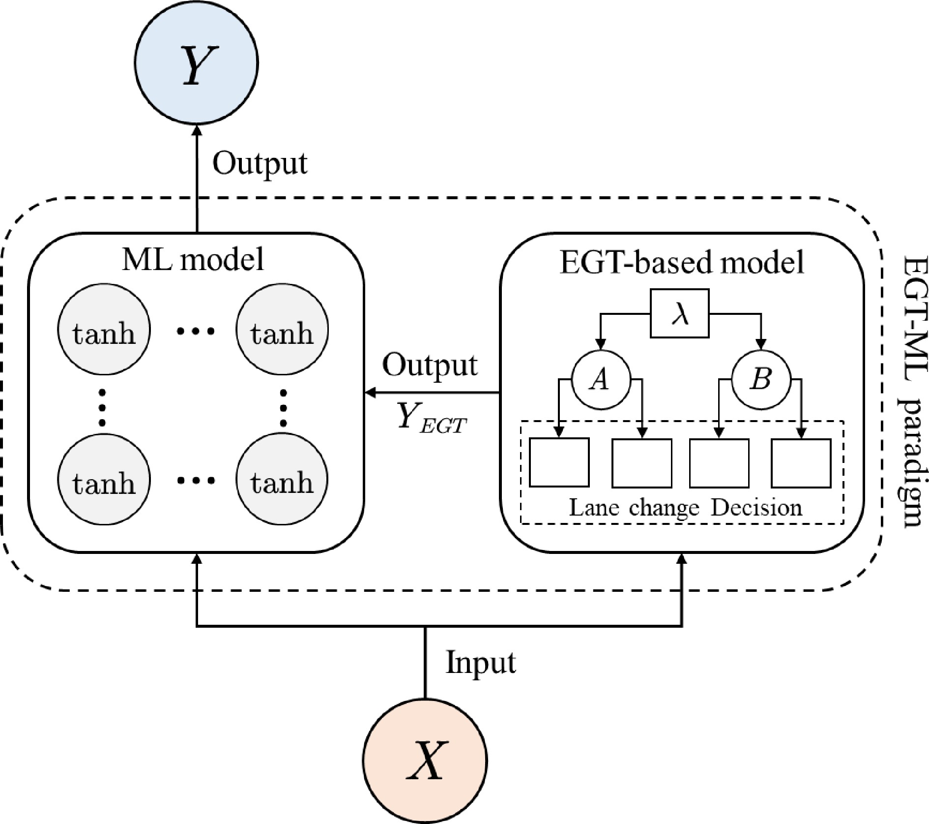
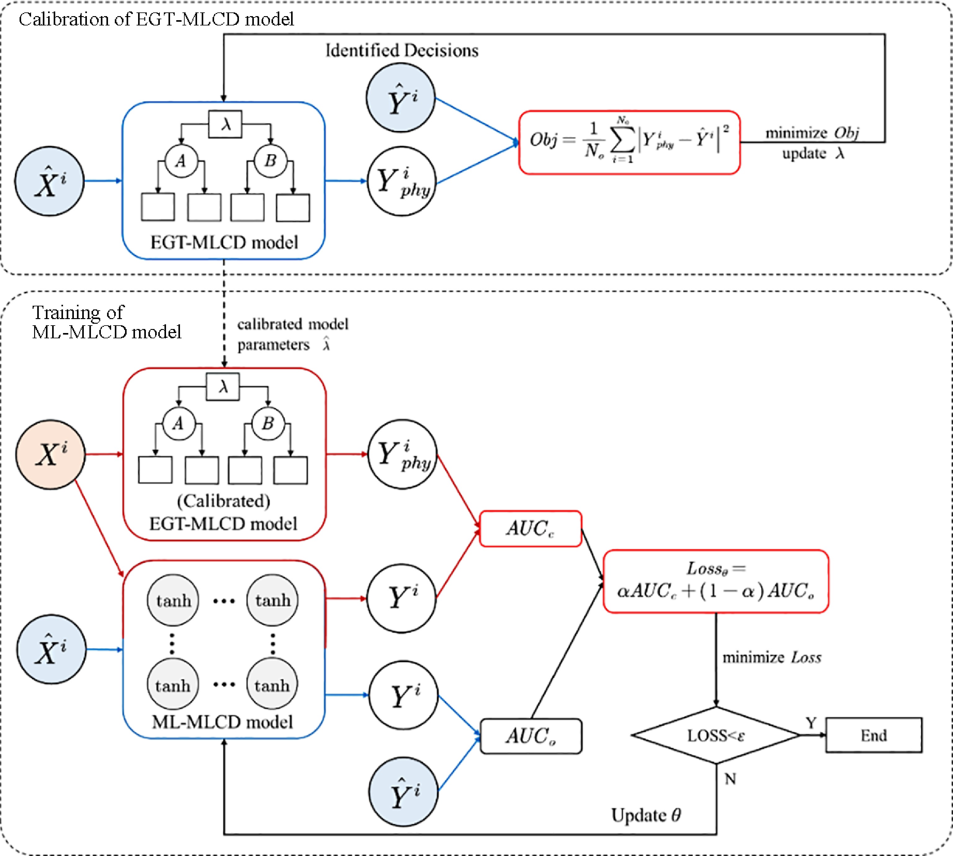
      To obtain a more predictive and explainable MLCD model that can depict the driving behavior of the interacted drivers with different driving styles, this study is aimed to develop an evolutionary game theory-based machine learning model (EGTML). The model prediction result is output by the machine learning model which is informed by the EGT-based physics model. The main contributions of this paper are as follows:

      (1) Design an EGTML architecture to model the mandatory lane change decision of multi-style drivers, which combines the physics-based model (data efficient and interpretable) and the machine learning model (high prediction accuracy).

      (2) Demonstrate the generalization of EGTML methods by using four different ML methods: ANN, RF, LightGBM, and XGBoost. The results showed that EGTML holds the potential to maintain high prediction accuracy and enhance the data-efficiency of training by incorporating physical knowledge.

      (3) Demonstrate the superiority of EGTML on real-world data. The results showed that the proposed hybrid paradigm outperforms the general machine learning model across various training data, especially when the data is sparse.

    • Since there are significant differences in driving behaviors of drivers with different styles, it is necessary to accurately model the lane-changing behaviors of drivers with different styles. This paper established a multi-style driver clustering model based on the Gaussian mixture model (GMM)[21].

    • Gaussian mixture model (GMM) is a linear combination of multiple single Gaussian models. If the d-dimensional vector x obeys the Gaussian mixture distribution, its probability density function is defined as:

      fM(x)=ki=1αi×f(xμi,Σi) (1)

      where, αi is the mixing coefficient, f(xμi,Σi) is the probability density function of the i-th Gaussian distribution, its equation is as follows:

      f(xμi,Σi)=1(2π)d2|Σ|12EXP[12(xμi)TΣ1i(xμi)] (2)

      where, μi is the d-dimensional mean vector, Σi is the d × d-dimensional covariance matrix. The main parameters of GMM are {(ai,μi,Σi)i=1,2,,k}. The Expectation-Maximum (EM) algorithm[22] is the common solution algorithm to obtain the optimal parameters. The EM algorithm continuously updates the parameters in the iterative process until the termination condition is satisfied.

    • During the operation of the vehicle by different styles of drivers, the operating parameters of the vehicle are different, which are intuitively reflected in the changes in parameters such as speed and acceleration[23]. The vehicle operating parameters can be obtained from the vehicle trajectory data. To consider the impact of the traffic operation state on drivers, define the ratio of vehicle speed to the space average speed as the speed ratio r to replace speed, the calculation formula is as follows:

      ri=vi¯vs (3)
      ¯vs=ni=1vin (4)

      where, ¯vb is the space average speed, n is the number of vehicles, and vi is the speed of ith vehicle. Based on the speed ratio r and the acceleration a, the driving style feature vector is constructed {E(r),VAR(r),E(a)}. The feature vector is brought into the GMM and the EM algorithm is used to obtain the optimal model parameters. Then, the vehicles are divided into k-clusters, corresponding to different driving styles.

    • Here, Evolutionary Game Theory (EGT)[24] is used to analyze the mandatory lane-changing decision game and predict the decision-making of game players. Dynamic analysis is used to solve the stable solution of the evolving system and predict the decision-making of the game participants. Two significant contents of EGT are shown as follows.

    • ESS is a strategy that enables the evolving system to reach a stable state, which is equivalent to Nash equilibrium in traditional game theory. Combined with the theory of biological evolution, ESS can be regarded as a process of survival of the fittest. Assuming that in a certain group, if the mutation of an individual can help the individual better adapt to the environment, the proportion of the mutation will increase, and the group can survive better. So, the mutation is the ESS of the group. In the MLCD game system, ESS is the decision made by drivers in the stable state.

    • 'Replication' refers to individuals following a better strategy, and the replicator dynamics equation indicates the rate of change in the proportion of individuals. The replicator dynamic equation is the differential equation defined as follows:

      dxidt=xi[u(si,x)u(s,x)] (5)

      where, si is the i-th strategy of the individual strategy set xi is the probability that the individual chooses the strategy si at time t, u(si, x) is the expected payoff when the individual chooses the strategy si, and u(s, x) is the average expected payoff of all strategy sets of the individual.

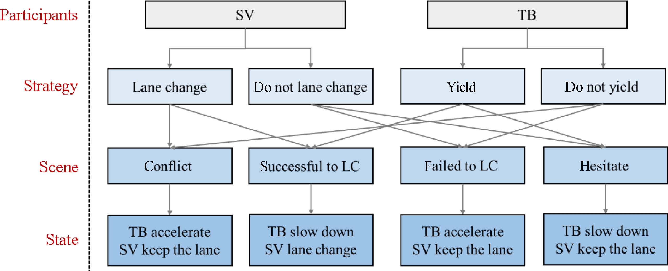
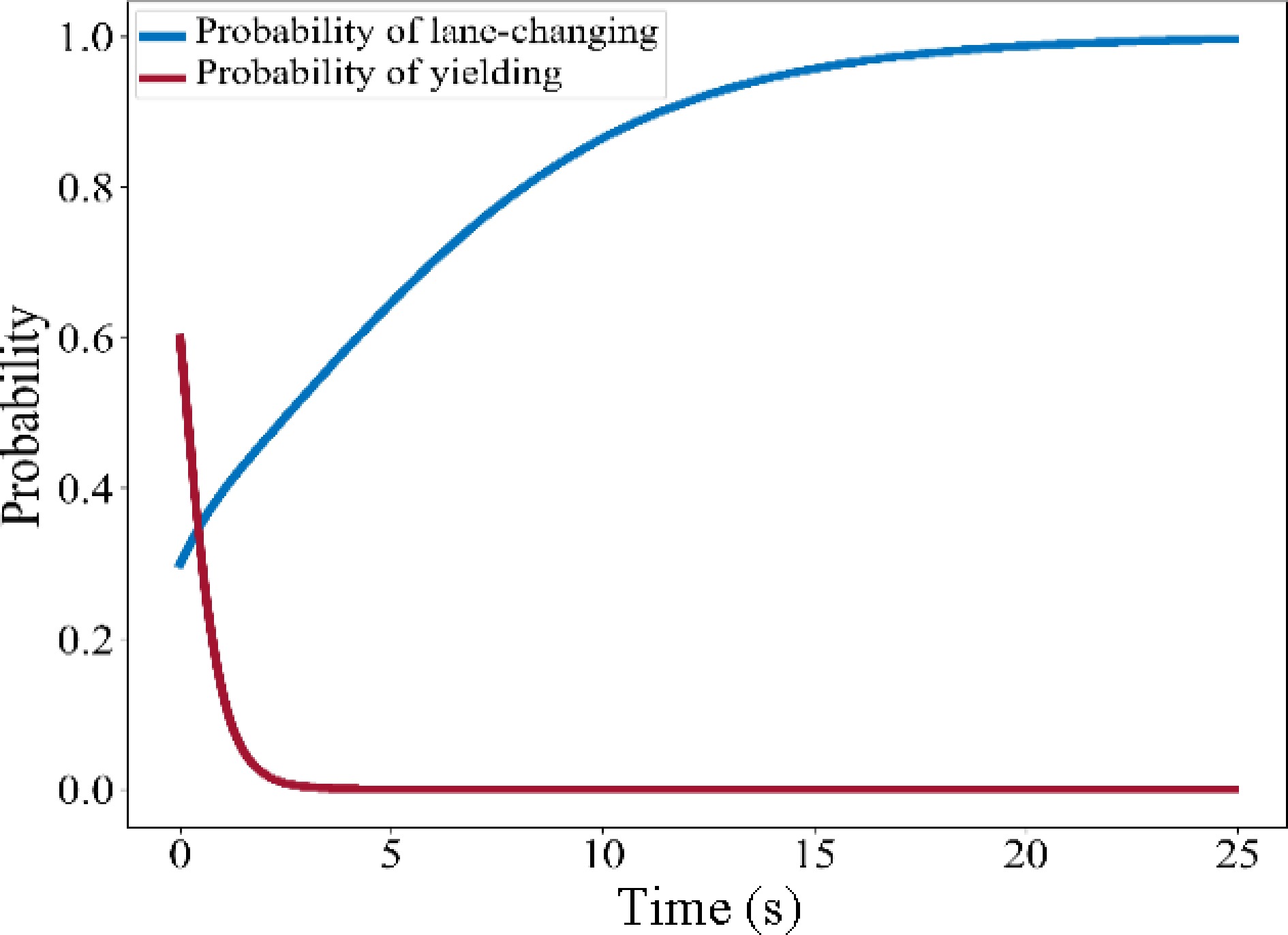
      As shown in Fig. 1, there are two players in the mandatory lane-changing decision game, the lane-changing vehicle (SV) and the vehicle behind it in the target lane (TB). According to the driving style of SV and TB, the MLCD game can be divided into different categories. First, SV signals the lane-changing request to TB. Second, TB responds by accelerating to refuse to yield or decelerating to yield. Finally, SV decides whether to lane change or not according to the response of TB.

      Figure 1. 

      The schematics of lane-changing.

    • SV and TB are the participants of the system, and the strategy set of SV is {Lane change, Do not lane change}, and the strategy set of TB is {Yield, Do not yield}. According to the different strategy combinations of SV and TB, the system will reach different stable states.

      The game process of the lane-change decision is shown in Fig. 2. Based on efficiency (i.e., speed loss), safety, and, accessibility (i.e., lane-changing demand), construct the payoff matrix for MLCD, which is shown in Table 1. P and Q denote the payoffs for SV and TB, respectively.

      Table 1.  The payoff matrix for MLCD.

      Game players SV
      Lane change No lane change
      TB Yield P11 : α1TTC + β1L P21 : −β1L
      Q11 : α2TTC − β2Δv Q21 : −β2Δv
      No yield P12 : −α1TTC P22 : −β1L
      Q12 : β2Δv − α2TTC Q22 : β2Δv

      Figure 2. 

      The game process of the lane-changing decision.

      Specifically, the efficiency payoff of TB is mainly reflected in the speed loss Δv caused by deceleration and yielding, and the payoff factor is β2. For the payoff of lane-changing demand, the distance of SV to the end of MLC L is used to represent the payoff of lane-changing demand, and the factor is β1. Time-To-Collision (TTC)[25] is used to represent the safety payoff between SV and TB, and the factors of SV and TB are α1 and α2 respectively. TTC refers to the time when the front and rear vehicles collide under the condition that the relative speed of the front and rear vehicles remain unchanged. It can be calculated as follows:

      TTC={yi1(t)yi(t)12(li1+li)vi(t)vi1(t)vi(t)>vi1(t)+vi(t)vi1(t) (6)

      where, yi(t), vi(t) and li represent the position, speed and length of the rear vehicle, yi-1(t), vi-1(t), and li-1 represent the position, speed, and length of the front vehicle. α1, α2, β1, and β2 are all in the range of (0,1) and satisfy α1 + β1 = 1 and α2 + β2 = 1.

    • SV and TB cannot take the optimal decision at the beginning of the game, so they must combine their own and each other's decisions, and eventually make the optimal decision through a game period and bring the system to a stable state. This optimal decision combination is the Evolutionarily Stable Strategy (ESS)[24].

      Suppose the probability of SV taking lane-changing behavior is x1, the probability of drivers taking yielding behavior is x2. The expected payoffs of SV and TB can be calculated.

      The expected payoff of SV taking lane-changing behavior is:

      W1=Ax2+C(1x2) (7)

      The expected payoff of SV not taking lane-changing behavior is:

      W2=Ex2+G(1x2) (8)

      The expected payoff of SV is:

      WSV=W1x1+W2(1x1) (9)

      The expected payoff of TB taking yielding behavior is:

      w1=Bx1+F(1x1) (10)

      The expected payoff of TB not taking yielding behavior is:

      w2=Dx1+H(1x1) (11)

      The expected payoff of TB is:

      wTB=w1x2+w2(1x2) (12)

      During the driving process, drivers will abandon low-payoff strategies and adopt high-payoff strategies. Therefore, x1 and x2 will change over time and satisfy the following equations:

      FSV(x1,x2)=dx1/dt=x1[W1WSV] (13)
      fTB(x1,x2)=dx2/dt=x2[w1wTB] (14)

      SV and TB cannot take the optimal decision at the beginning of the game, so they must combine their own and each other's decisions, through a period of game, and finally make the optimal decision, so that the system can reach a stable state. Assuming that at the beginning of the game, the probability of SV taking lane-changing behavior is x01, and the probability of TB taking yielding behavior is x02. Then, x01 changes to x11 according to Eqn (13), and x02 changes to x12 according to Eqn (14). After several iterations of this cycle, the system finally reaches a stable state, at this time, (xn1,xn2) is the stable point of the system, and the strategy combination is the ESS. When the system reaches a stable state, x1 and x2 satisfy the following equation:

      {x1(1x1)[(A+GCE)x2+CG]=0x2(1x2)[(B+FDF)x1+FH]=0x1,x2[0,1] (15)

      The four definite solutions of the equation are (0,0), (0,1), (1,0), (1,1), and another is (HFB+HDF,GCA+GCE). Not all of the above solutions can make the system reach a stable state. When the system reaches a stable state, the payoff function reaches the maximum value, so the stability analysis of solutions can be transformed into the problem of solving the maximum value of the function. For each solution, the dynamic equation is 0, so a solution satisfying the first derivative of the dynamic equation is less than 0 is a stable solution of the system. Therefore, the stable solution needs to satisfy the following equation:

      {FCV(x)=(12x1)[(A+GCE)x2+CG]<0fTB(x)=(12x2)[(B+HDF)x1+FH]<0 (16)

      Calculating the value of the first derivative of the dynamic equation at each solution, the results are as shown in Table 2.

      Table 2.  Stability analysis of equilibrium solution.

      (x1, x2) FCV(x) fTB(x) Stability
      (0, 0) C-G F-H Determined by the payoff matrix
      (0,1) A-E H-F
      (1,0) G-C B-D
      (1,1) E-A D-B
      (HFB+HDF,GCA+GCE) 0 0 Unstable solution

      Therefore, the set of stable solutions of the system is {(0,0), (0,1), (1,0), (1,1)}, and the corresponding set of ESS is {(Do not lane change, Do not yield), (Do not lane change, Yield), (Lane change, Do not yield), (Lane change, Yield)}. The stable solution of the system is determined by the payoff matrix. Finally, EGT-based MLCD is determined by the payoff matrix and the initial values of x1 and x2 according to the identified decisions. Assuming the stable solution of the system is (1,0), then solve the ESS of the system and calculate the values of x1 and x2 to determine the lane-changing decision of SV. The evolution path of the system is shown in Fig. 3.

      Figure 3. 

      Schematic diagram of the evolution of the probability.

      In this case, SV has a greater payoff by lane-changing, but TB tends to choose not to yield, the players compete for the road resources and the ESS is (Lane change, No yield).

    • Whether SV changes the lane or not depends not only on the probability of SV lane-changing, but also the probability of TB yielding, but also on whether the lane-changing safety criteria are satisfied[26]. Because TTC can reflect the relative motion trend and collision possibility between the front and rear vehicles, it is utilized to formulate the lane-changing safety criteria and shown as follows:

      TTCTFTTCminTF,TTCTBTTCmin TB (17)

      where, TTCTF and TTCTB are between SV and TF, TB, TTCminTF and TTCminTB are constraints.

    • Only when the probability of SV lane-changing and the probability of TB yielding are both greater than 0.5 and the lane-changing safety criteria is satisfied, the model outputs YEGT = 1, indicating SV lane changing, otherwise, the model outputs YEGT = 0, indicating SV no lane changing. The EGT-based physics model is as follows:

      YEGT={1p1>0.5,p2>0.5,TTCTF>TTCminTF,TTCTB>TTCminTB0otherwise (18)
    • According to the PIDL architecture proposed by Mo et al.[19], the EGTML model consists of two elements: a machine-learning model and an EGT-based physics model. Both models take the feature vector X as input and the lane-changing decision Y as output. The output of the EGTML model is the output of the ML model, and the output of the EGT-based model is the physical knowledge of ML model, which provides constraints for the output of the ML model. Figure 4 illustrates the structure of the EGTML model.

      Figure 4. 

      Structure diagram of EGTML.

    • In previous MLCD models, the features such as speed, acceleration, and speed difference are generally selected. But the traffic state information contained in these features is not comprehensive to fully describe the complex interaction between SV and surrounding vehicles (i.e., front vehicle on the target lane TF, behind vehicle on the target lane TB, front vehicle on the current lane CF, behind vehicle on the current lane CB). This paper comprehensively considered the safety indicators TTC, and finally determined 24 features to construct the feature vector X as the input of the EGTML model, as shown in Table 3.

      Table 3.  Features of the EGTML model.

      Symbol Meaning Unit
      VOV, VOF, VOB, VTP, VTH The speed of the vehicle m/s
      AOV, AGF, ACB, ATF, ATB The acceleration of the vehicle m/s2
      ΔVCF, ΔVCB, ΔVTF, ΔVTB The speed difference between vehicles m/s
      GCF, GCB, GTF, GTB The gap between vehicles m
      TTCCF, TTCCB, TTCTF, TTCTB The TTC between vehicles s
      L The distance of SV to the end of MLC m
      ¯vs Space average speed m/s
    • The observation dataset is a set of state-decision pairs {X,ˆY}, where the observed state is the feature vector X, and the identified decision is ˆY, where ˆY=1 indicates lane change and ˆY=0 indicates no lane change. In addition to the observation dataset, the collocation dataset needs to be defined. The collocation dataset is a set of state-decision pairs {X,YBGT}, where the observed state is the feature vector X, and the collocation decision Ytar  is the lane-changing decision predicted by EGT-based physics model for the observed state. According to a certain training-test split ratio, observation dataset is divided into two subsets. One subset and the collocation dataset constitute the training dataset, and the other subset is used for model testing. The process of the split dataset is shown in Fig. 5.

      Figure 5. 

      Relationship between observation and collocation dataset.

    • After the dataset is divided, the loss function of the model needs to be defined. The loss function consists of two parts, one of which is the difference between the identified decision and the predicted decision of the machine learning model (i.e., the data difference), and another is the difference between the predicted decision of EGT-based model and the machine learning model. (i.e. the physics difference). Specifically, the AUC value is used to evaluate the difference. The loss function is defined as follows:

      Lossθ=αAUCc+(1α)AUCo (19)

      where, α is the weight that balances the contributions made by the data difference and physics difference.

    • The trained EGTML can be used to predict the test dataset. Precision (P), recall (R), and accuracy (A) are used to evaluate the prediction performance of the EGTML model. The indexes are defined as follows:

      P=TPTP+FP (20)
      P=TPTP+FP (21)
      A=TP+TNTP+FP+TN+FN (22)
    • The model training process of EGTML consists of two processes, EGT-based model parameter calibration and machine-learning model parameter optimization. The training process is shown in Fig. 6. The EGT-based model parameter calibration problem can be written as the following optimization problem:

      Figure 6. 

      Training process of EGTML.

      minλObj=1NoNoi=1|YiphyˆYi|2i=1,,N0 s.t. Yiphy=fλ(^Xi|λ),λΛ (23)

      where, λ are the parameters of the EGT-based model, N0 is the number of observed data, YiEOH is the ith predicted decision by the EGT-based model ˆYi is the ith identified decision Λ is the feasible domain of the parameters, representing the physical range of each parameter. The objective function obj calculates the difference between the predicted decision of the EGT-based model and the identified decision in MSE form. The smaller the objective function, the closer the model result is to the observed result.

      After the parameter calibration of the EGT-based model, using Eqn (19) to calculate the loss between the predicted decision of the ML model and the predicted decision of the EGT-based model, the identified decision, respectively, to obtain the loss of EGTML. The Adam algorithm is used to minimize the loss until the algorithm obtains the optimal parameter θ.

    • The performance of the EGTML model is validated using the real-world data, US-101 dataset in the Next Generation SIMulation (NGSIM) dataset[27]. The collection section of the US-101 dataset was the southbound section of the US-101 Freeway in Los Angeles, California, USA. The length of the road section was 640 m, including five mainline lanes, an on-ramp, an off-ramp, and a distribution lane. The five mainline lanes from the inner lane to the outer lane were numbered sequentially from lane 1 to lane 5, the distribution lane is lane 6, the on-ramp and off-ramp are lane 7 and lane 8. The trajectory data in US-101 is the original unfiltered data, and there were outliers and measurement errors, which will affect the training and validation of the model. Therefore, the moving average method is used to smooth the position, speed, and acceleration of the vehicle to improve the data quality and reduce error interference[28] .

      The continuous data in the dataset is then binned to enhance the robustness and reduce the risk of model overfitting. In the US-101 data collection section, there were a lot of mandatory lane-changing behaviors in lane 5 and lane 6. Five hundred and eighty six samples were extracted and the start and end times of each sample were identified. When the lateral speed was greater than 0.2 m/s, there was a tendency to move laterally into an adjacent lane within 1 s, which was defined as the start time. When the lateral speed was less than 0.2 m/s and the lateral position remained stable within 1 s, this was defined as the end time[29]. Lateral refers to the direction perpendicular to the direction of the lane. Taking vehicle No. 20 as an example, the identification of the start and end time of lane-changing is shown in Fig. 7. After identifying the start time and the end time, the trajectory data of 5 s before the start time and the entire lane-changing process is selected to simplify the dataset.
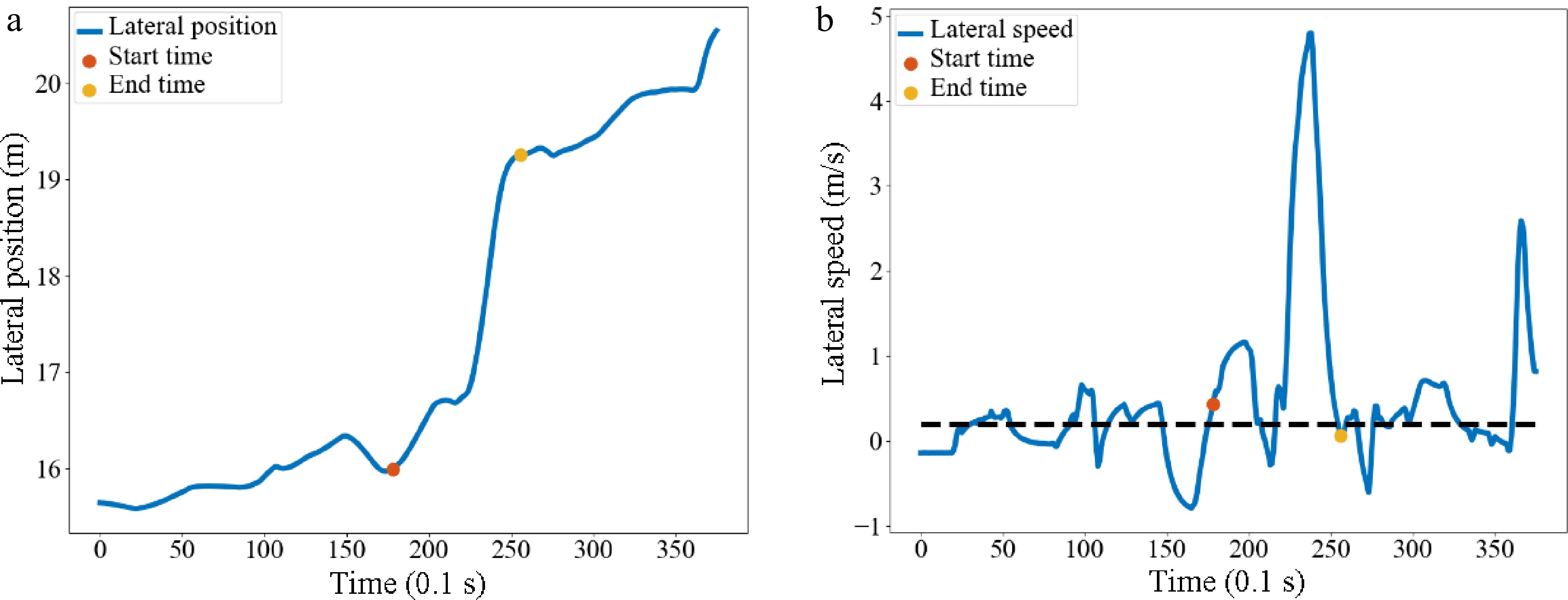
      Figure 7. 

      Identification of the start and end time of vehicle No. 20. Diagram of (a) lateral position, (b) lateral speed.

    • The number of cluster centers of GMM was defined as 2, and the drivers on lane 5 and lane 6 were divided into two data subsets, corresponding to conservative drivers, and aggressive drivers respectively. The number of aggressive drivers was 616, accounting for 37.84%, and the number of conservative drivers was 1,012, accounting for 62.16%. Overall, both the average acceleration and the variance of speed ratio of aggressive drivers were larger than those of the conservative drivers. The distribution of sample eigenvalues are shown in Fig. 8. It can be seen that both the average acceleration and the variation of speed ratio of aggressive drivers are larger than those of the conservative drivers.
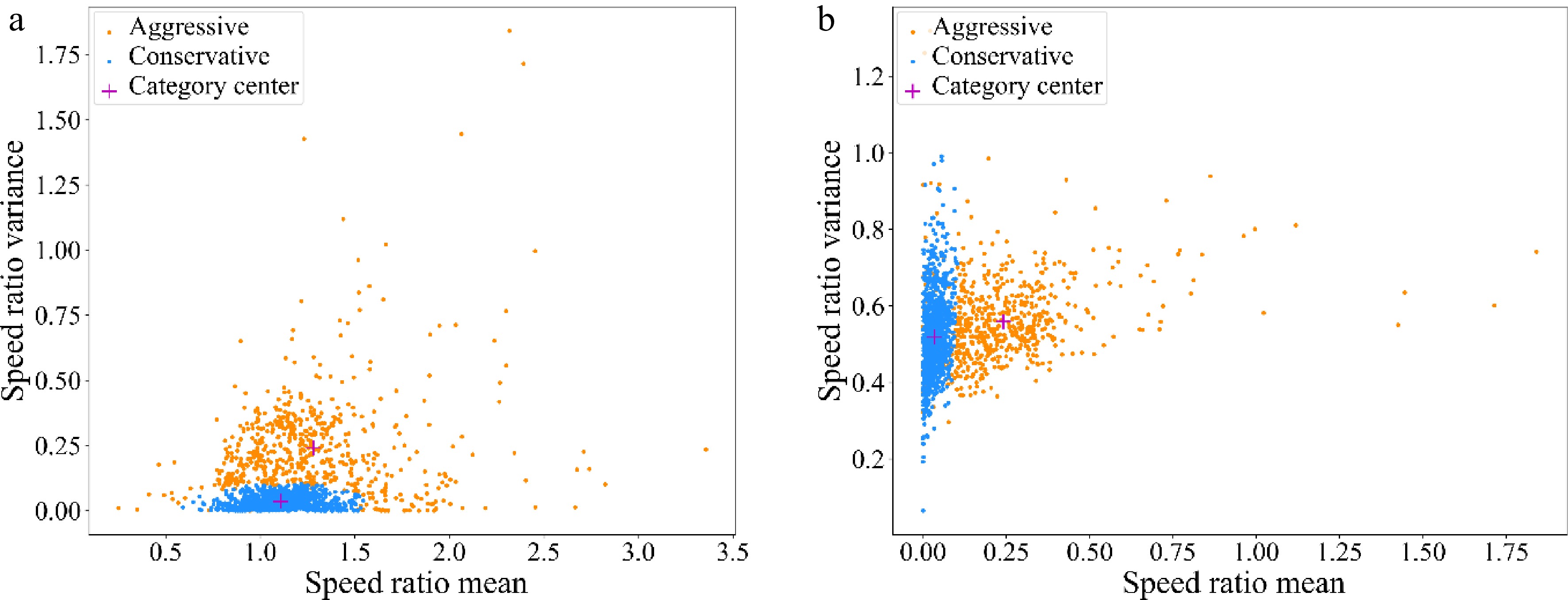
      Figure 8. 

      Distribution of sample eigenvalues. (a) Speed ratio mean - Speed ratio variance; (b) Speed ratio variance - Acceleration mean.

    • According to the driving style of SV and TB, the MLCD game can be divided into the following four categories: Category 1 is the aggressive SV and aggressive TB. Category 2 is the aggressive SV and conservative TB. Category 3 is the conservative SV and aggressive TB. Category 4 is the conservative SV and conservative TB. Using observation data to calibrate the EGT-based model parameters for four categories. For the payoff factors, in the range of (0,1), with a step size of 0.01, all the parameter combinations were traversed to optimize Eqn (23), and the calibration results are shown in Table 4. The definition of each parameter is described above. The 85th percentile TTCTF and TTCTB were chosen as the calibrated values for TTCminTF and TTCminTB to ensure the safety performance of most vehicles.

      Table 4.  The calibration of parameters.

      Category 1 2 3 4
      α1 0.98 0.99 0.96 0.97
      β1 0.02 0.01 0.04 0.03
      α2 0.8 0.9 0.8 0.85
      β2 0.2 0.1 0.2 0.15
      TTCminTF 6.25 6.25 6.25 6.25
      TTCminTB 6.25 6.25 6.25 6.25

      After parameter calibration, the payoff matrix was calculated and the evolution with time of the probability of lane-changing and yielding for each of the four MLC categories calculated by replicator dynamic equations and was plotted in Fig. 9.
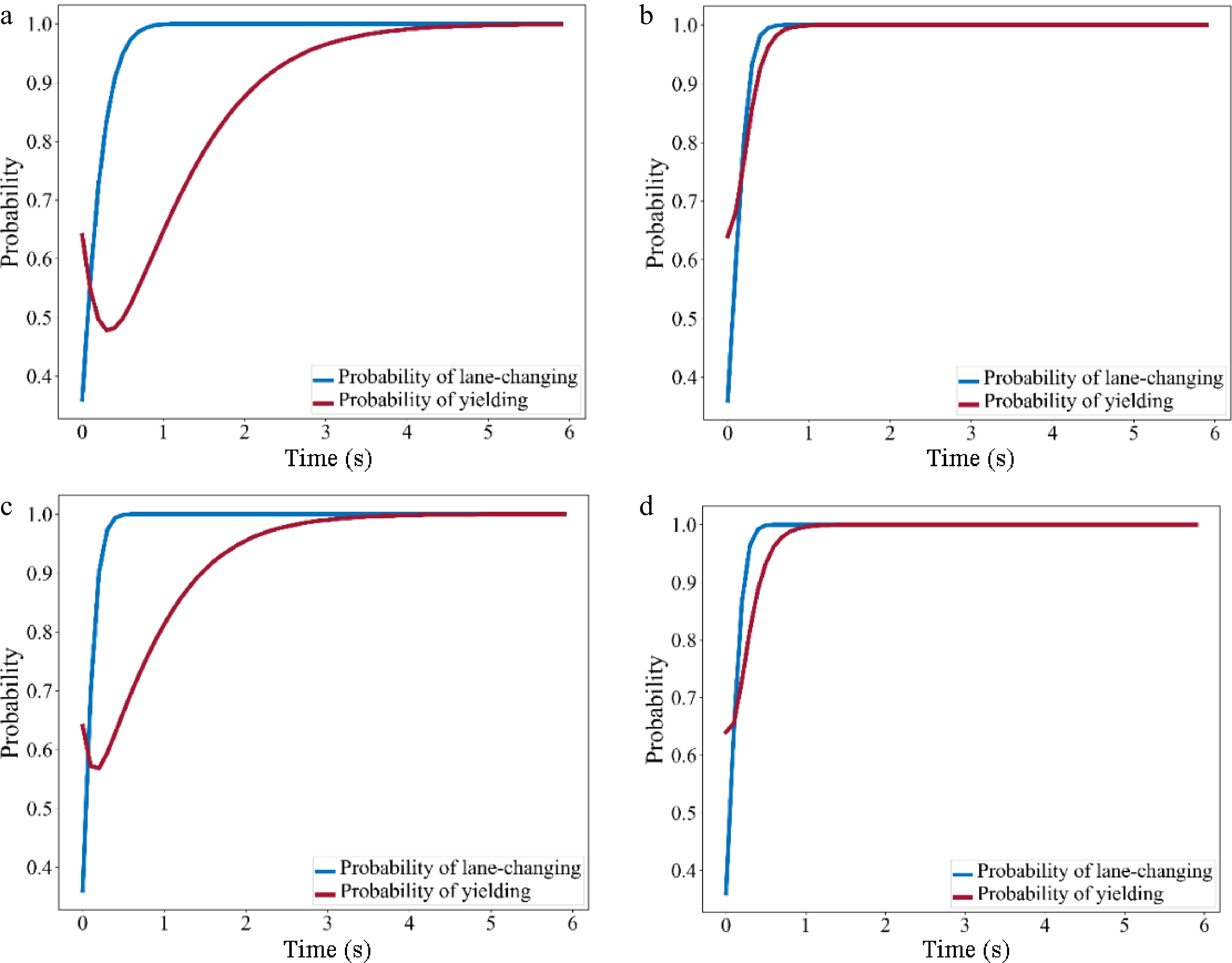
      Figure 9. 

      Evolution diagram of probability of lane-changing and yielding. (a) Category 1 (Aggressive SV - Aggressive TB); (b) Category 2 (Aggressive SV - Conservative TB); (c) Category 3 (Conservative SV - Aggressive TB); (d) Category 4 (Conservative SV - Conservative TB).

      In Fig. 9a & c, the probability of SV lane-changing increased over time, while the probability of TB yielding decreased at first and then increased gradually, implying that there may be an obvious competition between two drivers at the beginning of the game when TB is aggressive. Compared to aggressive SV, when SV is conservative, the intensity and duration of the competition was comparatively lower.

      In Fig. 9b & c, the probability of SV lane-changing increases more rapidly, while the probability of TB yielding increases directly. That is, conservative TB tends to yield to SV during the game.

    • The prediction performance on the test dataset of the EGTML model was evaluated by precision (P), recall (R), and accuracy (A). Widely-used ML models (i.e., ANN, RF, LightGBM, and XGBoost) were applied to construct the EGTML model.

      ANN[30]: Artificial neural network (ANN) is a computational model that consists of several processing elements that receive inputs and deliver outputs based on their predefined activation functions.

      RF[31]: Random Forest (RF) is an ensemble learning method for classification that operates by constructing a multitude of decision trees during the training process. The output of the RF is the class selected by most trees.

      LightGBM[32]: LightGBM is an improvement of gradient ascending algorithm (GBDT) in efficiency and scalability, which incorporates two innovative techniques: Gradient-based One-Side Sampling (GOSS) and Exclusive Feature Bundling (EFB).

      XGBoost[33]: XGBoost is a scalable, distributed gradient-boosted decision tree (GBDT) that provides parallel tree boosting.

      The evaluation of different ML models is shown in Table 5. The ROC curves, and PR curves are shown in Fig. 10. It can be seen that the EGTML models using different ML models all have good prediction performances, among them, the LightGBM performs the best.

      Table 5.  The evaluation of different ML models.

      Index ANN RF LightGBM XGBoost
      P 0.775 0.855 0.833 0.871
      R 0.963 0.931 0.944 0.933
      A 0.795 0.832 0.865 0.847

      Figure 10. 

      The ROC curves, and PR curves of different ML models. (a) ROC curves; (b) PR curves.

    • After applying the best performing ML model (i.e., LightGBM), the distribution of longitudinal Lane Change Decision position output from EGTML (EGT-LightGBM) and LightGBM, as well as the identified decisions (i.e., ground truth), were plotted and are shown in Fig. 11 by MLC game categories.
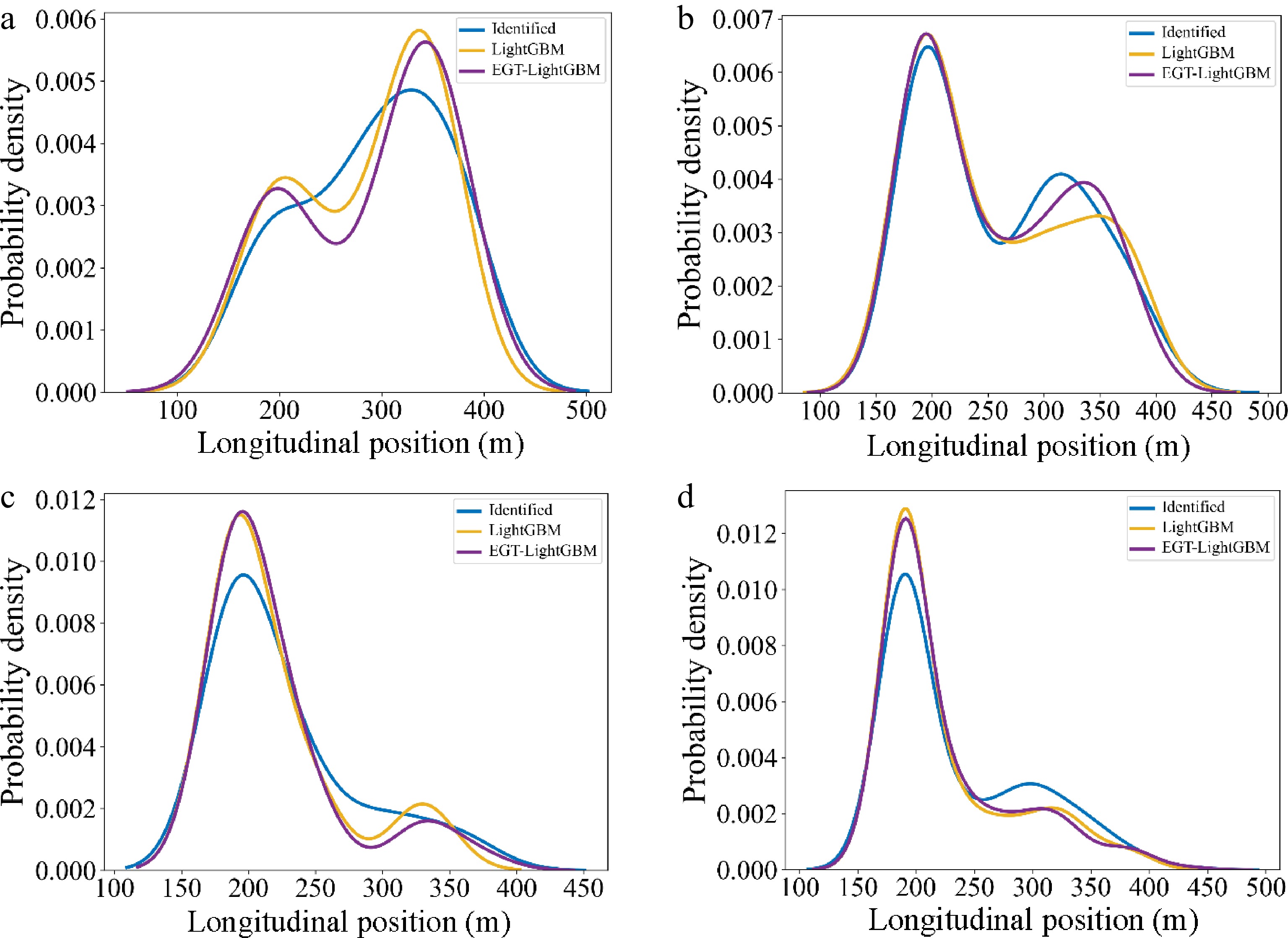
      Figure 11. 

      Distribution of longitudinal Lane Change Decision position. (a) Category 1 (Aggressive vs Aggressive); (b) Category 2 (Aggressive vs Conservative); (c) Category 3 (Conservative vs Aggressive); (d) Category 4 (Conservative vs Conservative).

      Category 1 (Aggressive vs Aggressive): In Fig. 11a, it can be seen that the distribution of output from EGTML is more similar than that from the pure ML model. This result is also confirmed by the KL divergence gained from pure ML and ground truth (i.e., 0.271) as well as from EGTML and ground truth (i.e., 0.231). According to Fig. 11a, the competition between two aggressive drivers may increase the difficulty of MLC, which leads to the discrete distribution of lane change positions.

      Category 2 (Aggressive vs Conservative): KL divergence from EGTML (i.e., 0.081) is lower than that from ML (i.e., 0.098). In Fig. 11b & c, because conservative drivers tend to yield to aggressive drivers during the game, more aggressive drivers can finish their MLC earlier than that in Category 1.

      Category 3 (Conservative vs Aggressive): KL divergence from EGTML (i.e., 0.145) is lower than that from ML (i.e., 0.172). According to the low intensity and duration of the competition from conservative SV and aggressive TB in Fig. 9c, the difficulty of MLC for conservative drivers is higher than that of Category 4 (i.e., the distribution of lane change positions in Category 4 is more centralized).

      Category 4 (Aggressive vs Conservative): Both the tendency of distribution in Fig. 11d and KL divergency (i.e., 0.036 > 0.029) demonstrate that EGTML has a better performance in the prediction of MLCD. Because the tendency of evolution probability of SV and TB in Fig. 9d is similar to that in Fig. 9b, a comparable trend of the output distribution is also displayed between Fig. 11d & b.

      In summary, EGTML can learn the knowledge of evolutionary game theory and capture the game interactions between multi-style drivers in different game scenarios, which improves the interpretability of traditional ML.

    • EGT-LightGBM was used for testing the parameter sensitivity of EGTML.

      Firstly, to show that the advantages of the EGTML model persist across different numbers of training data, different numbers of training data wer randomly selected and the prediction performances evaluated on the test dataset. The results are shown in Fig. 12a, where the x-axis is the number of training data, and the y-axis is the prediction accuracy. As can be seen, the overall performance of the EGTML model is better than the traditional ML model and the EGT-based model even with the variability of the training data. The difference with the former shrinks and the difference with the latter increases as the training data increases. This phenomenon is similar to the results shown by PINN-CF[19].

      Figure 12. 

      The performance of EGTML. (a) Varying numbers of training data; (b) varying α.

      Secondly, to analyze the influence of the weight α on the EGTML model, the model is trained by the value of α from 0 to 1 with a step size of 0.1. Then, the performance of the trained model is evaluated on the same test dataset. The results are shown in Fig. 12b, the x-axis is the value of α, and the y-axis is the prediction accuracy. As can be seen, when the value of α is 0.1, the performance of the EGTML model is optimal.

    • This paper develops an evolutionary game theory-based machine learning mandatory lane change decision model (EGTML). The prediction result is output by the machine learning model which is informed by the EGT-based physical model. This modeling framework holds the potential to maintain high prediction accuracy and enhance the data efficiency of training by incorporating physical knowledge. The generalization of the EGTML method is further validated using four machine learning models: ANN, RF, LightGBM, and XGBoost, and the superiority of EGTML is demonstrated on the NGSIM dataset. Applying the best-performing EGT-LightGBM, and LightGBM to test the parameter sensitivity of EGTML, the results show that the EGTML model outperforms the general ML model, especially when the data is sparse.

      To the best of our knowledge, this paper is the first-of-its-kind that employs a hybrid paradigm where a physics-based model is encoded into a machine learning model for mandatory lane-changing decision prediction. Thus, there are still a lot of unresolved research questions. This work will be extended in several directions. (1) More advanced physics-based MLCD models will be encoded into ML models, which may hold the potential to capture more complex lane-changing behaviors. (2) A systematic simulation procedure should be developed for testing the proposed EGTML model and identifying the best physics-based models by deriving some key metrics (e.g., collision rate, conflicting distribution).

    • The authors confirm contribution to the paper as follows: conceptualization, methodology, draft manuscript preparation: Xu S; software: Xu S, Li M; data curation: Li M; visualization, investigation: Li M, Zhou W, Zhang J; supervision, project administration, funding acquisition: Wang C. All authors reviewed the results and approved the final version of the manuscript.

    • Data will be made available upon reasonable request to the corresponding author.

      • This research was supported by the National Key R&D Program of China (2023YFE0106800), and the Postgraduate Research & Practice Innovation Program of Jiangsu Province (SJCX24_0100).

      • The authors declare that they have no conflict of interest. Chen Wang is the Editorial Board member of Digital Transportation and Safety who was blinded from reviewing or making decisions on the manuscript. The article was subject to the journal's standard procedures, with peer-review handled independently of this Editorial Board member and the research groups.

      • Copyright: © 2024 by the author(s). Published by Maximum Academic Press, Fayetteville, GA. This article is an open access article distributed under Creative Commons Attribution License (CC BY 4.0), visit https://creativecommons.org/licenses/by/4.0/.
    Figure (12)  Table (5) References (33)
  • About this article
    Cite this article
    XU S, LI M, ZHOU W, ZHANG J, WANG C. 2024. An evolutionary game theory-based machine learning framework for predicting mandatory lane change decision. Digital Transportation and Safety 3(3): 115−125 doi: 10.48130/dts-0024-0011
    XU S, LI M, ZHOU W, ZHANG J, WANG C. 2024. An evolutionary game theory-based machine learning framework for predicting mandatory lane change decision. Digital Transportation and Safety 3(3): 115−125 doi: 10.48130/dts-0024-0011

Catalog

  • About this article

/

DownLoad:  Full-Size Img  PowerPoint
Return
Return