-
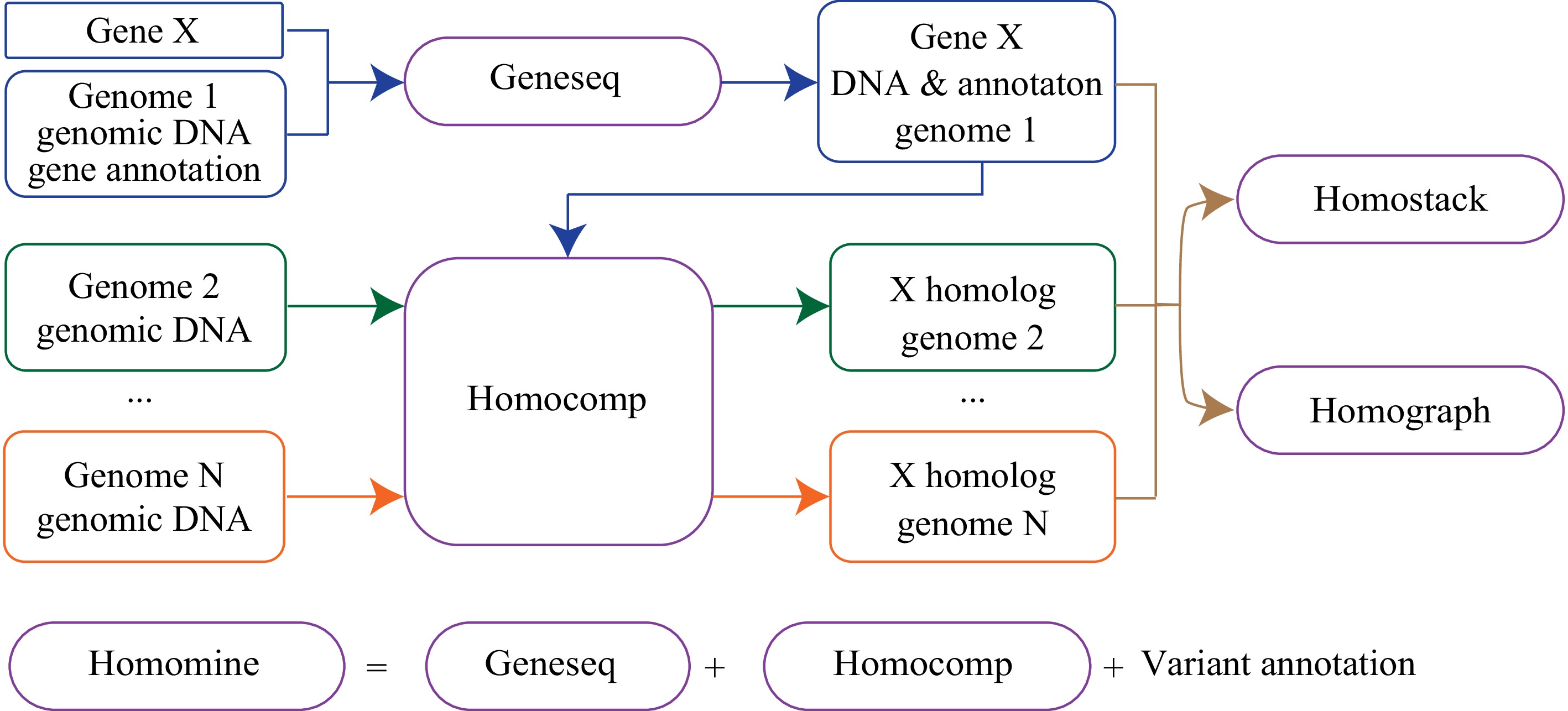
Figure 1.
Overview of Homotools. Module geneseq extracts sequences and related information from databases for a gene (e.g., gene X); homocomp implements homolog searching for gene X and visualizes the comparison of two homologs; homograph determines haplotypes of multiple homologs, and displays an alignment graph of a set of homologs; and homostack stacks input sequences and shows alignments; Module homomine is a pipeline implementing modules geneseq and homocomp for homologous searching and annotating all variants between the query sequence and the resulting homolog.
-
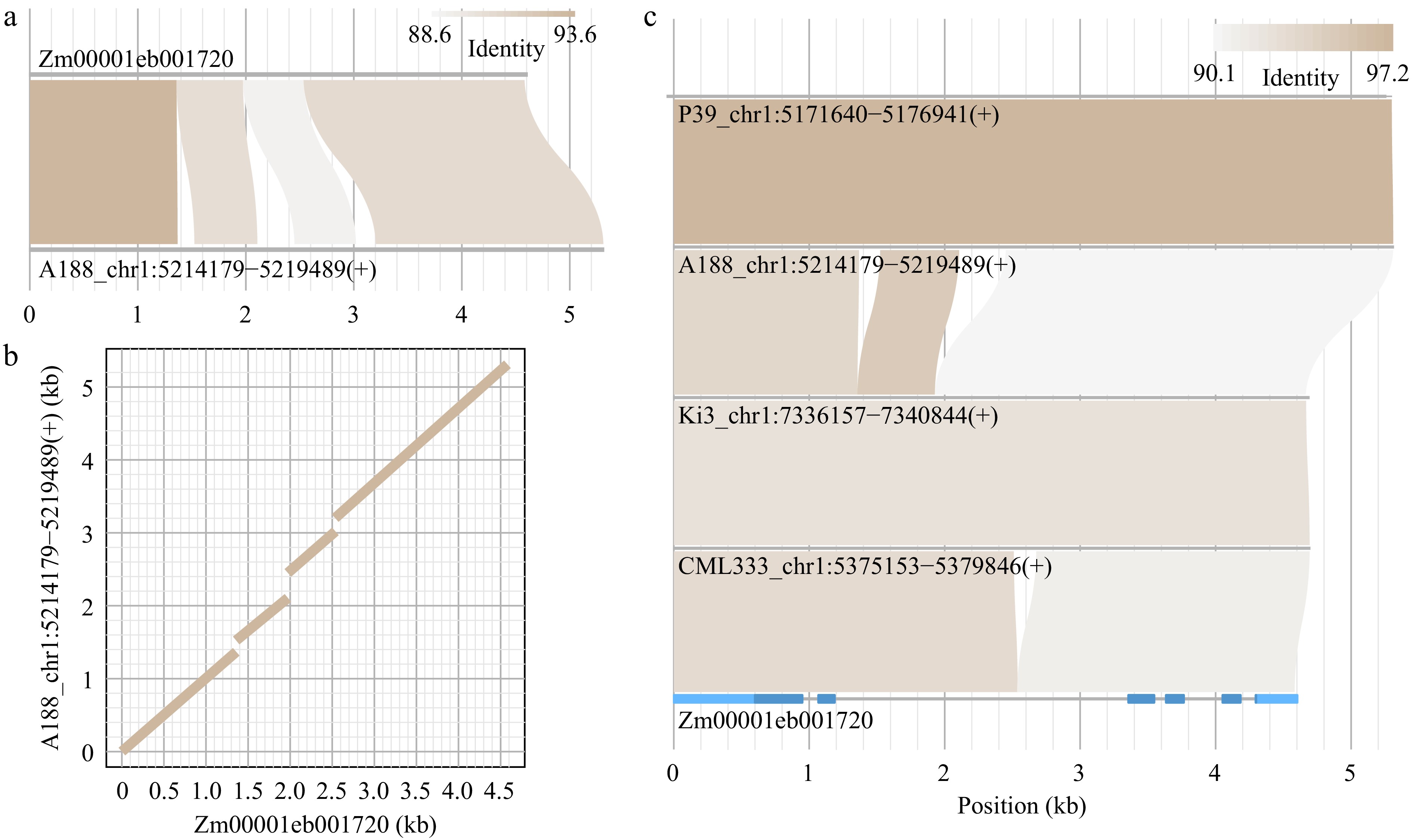
Figure 2.
Alignment visualization via homocomp and homostack. (a), (b) A target homologous sequence of the query sequence (Zm00001eb001720) was identified in the A188 genome using module homocomp. (a) An alignment plot, and (b) a dotplot were output. (c) Multiple sequences retrieved by homocomp, along with the query sequence, were supplied to homostack to show the sequential alignments. The gene structure of Zm00001eb001720 was plotted, in which light and dark blue represent untranslated exon regions and coding regions, respectively.
-
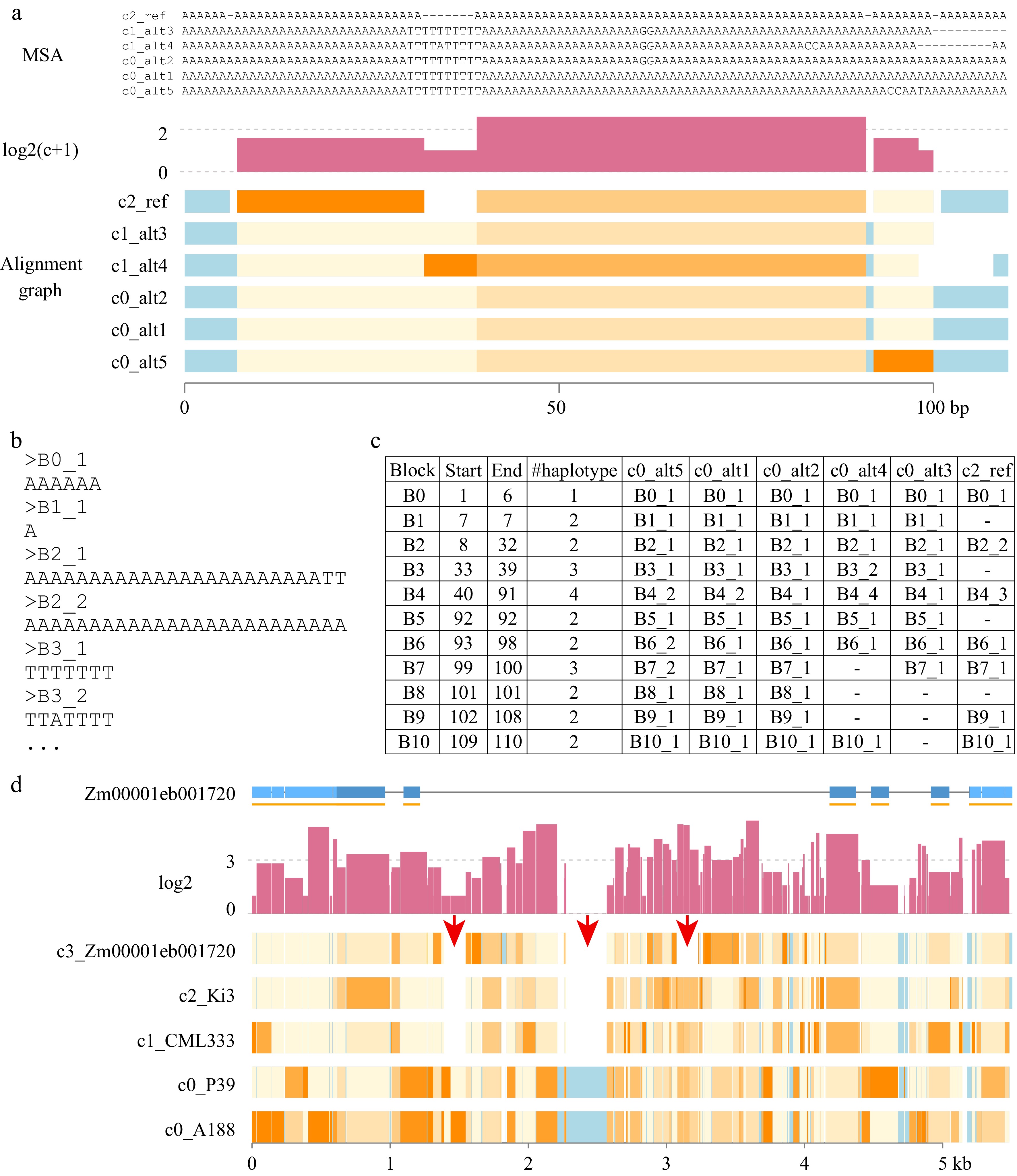
Figure 3.
Homograph outputs. (a) Three parts are included: MSA, log2(c+1), and Alignment graph. MSA displays a graphic view of multiple sequence alignment (MSA) for helping understand the alignment graph. The MSA was divided into blocks at the transition between a gap ('-') and a nucleotide base. For each block, the single nucleotide substitution sites, excluding gaps, were counted. The Y-axis unit is at the scale of log2 of (c) the substitution count, which is adjusted by adding 1. In the alignment graph, each rectangle represents an alignment block without a gap. Light blue represents conserved regions with no substitution polymorphisms. The gradient colors from light yellow to orange indicate the divergent levels from the consensus sequences, from low divergence to high divergence, respectively. Names of taxa are prefixed with cluster groups (e.g., c0). (b) The allele sequence of each block is stored in a FASTA file. (c) A table output lists the allele type of each taxon at each block. The Start and End coordinates are the MSA alignment positions. The number of haplotypes (#haplotype) specifies the number of alleles of a block, which includes the allele of a gap if it exists. (d) A graphic output of homograph analysis of knox1 homologs. Red arrows point at regions with presence and absence variation. The gene structure of Zm00001eb001720 was plotted, in which light and dark blue represent untranslated exon regions and coding regions, respectively. Each orange line under the gene structure indicates an exon, which could be split by alignment gaps.
-
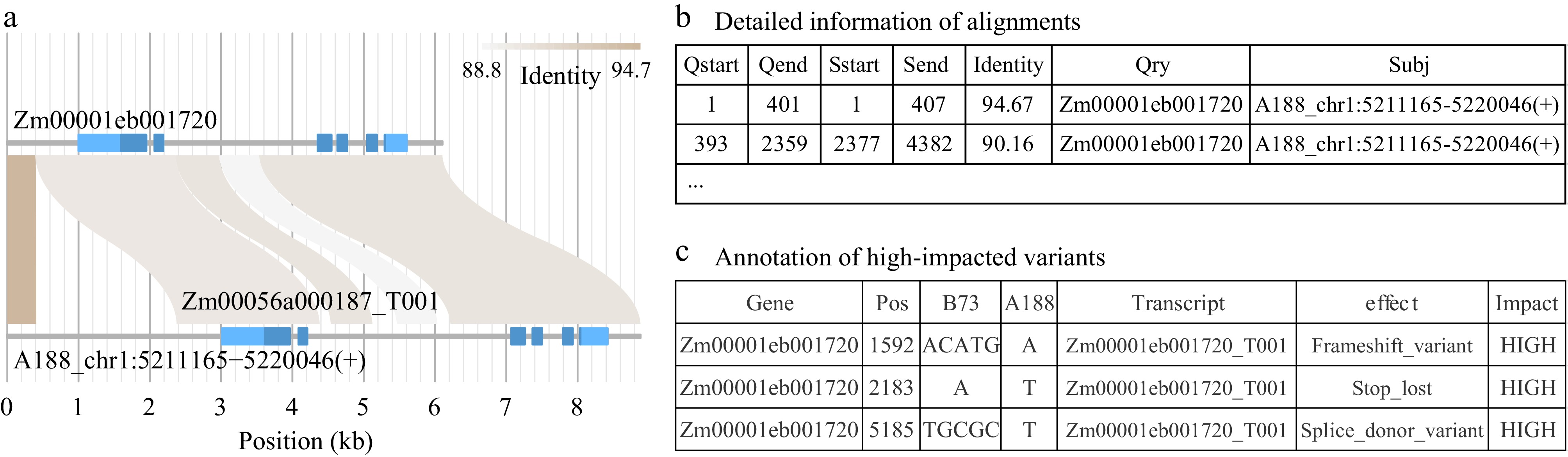
Figure 4.
Partial outputs from module homomine. (a) Homomine searches homologous sequences of a query gene Zm00001eb001720 in a targeted genome (A188). The flanking 1 kb on the 5’ end and 500 bp on the 3’ end are included. Homomine identifies the matching region that harbors Zm00056a000187 in the A188 genome. Light and dark blue in gene structures represent untranslated exon regions and coding regions, respectively. (b) In the homomine output, detailed alignments between the two homologs are provided. (c) The homomine output lists variants identified between the two homologs, including structural variation. Variants are annotated and moderate- and high-impacted variants are highlighted in the output. The table shows the annotation of variants with a high impact.
-
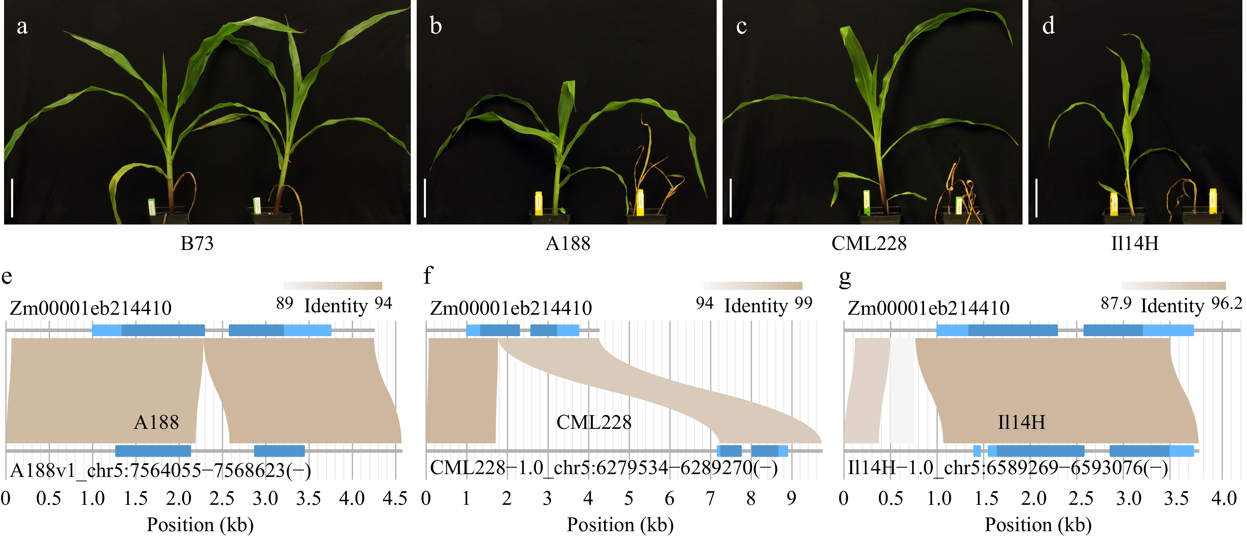
Figure 5.
Phenotypic results of nicosulfuron treatments and allelic comparisons. (a)−(d) Maize plants with nicosulfuron treatment at a dose of 137 gram active ingredient per hectare (right) and a mock treatment (left). Bar = 10 cm. (e)−(g) The structural comparison between each allele of A188, CML228, and Il14H with the B73 allele of gene Zm00001eb214410. Light and dark blue in gene structures represent untranslated exon regions and coding regions, respectively.
Figures
(5)
Tables
(0)