-
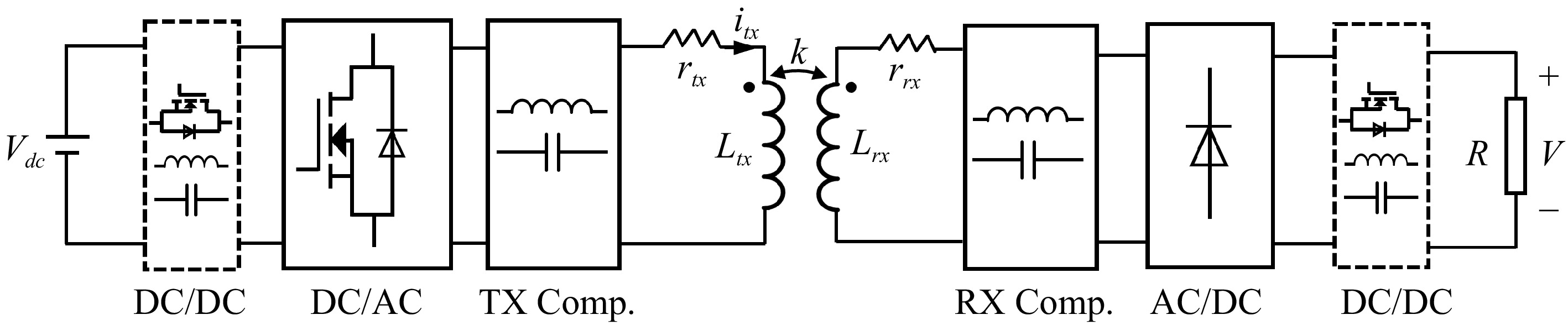
Figure 1.
Configuration of 1TX-1RX system.
-
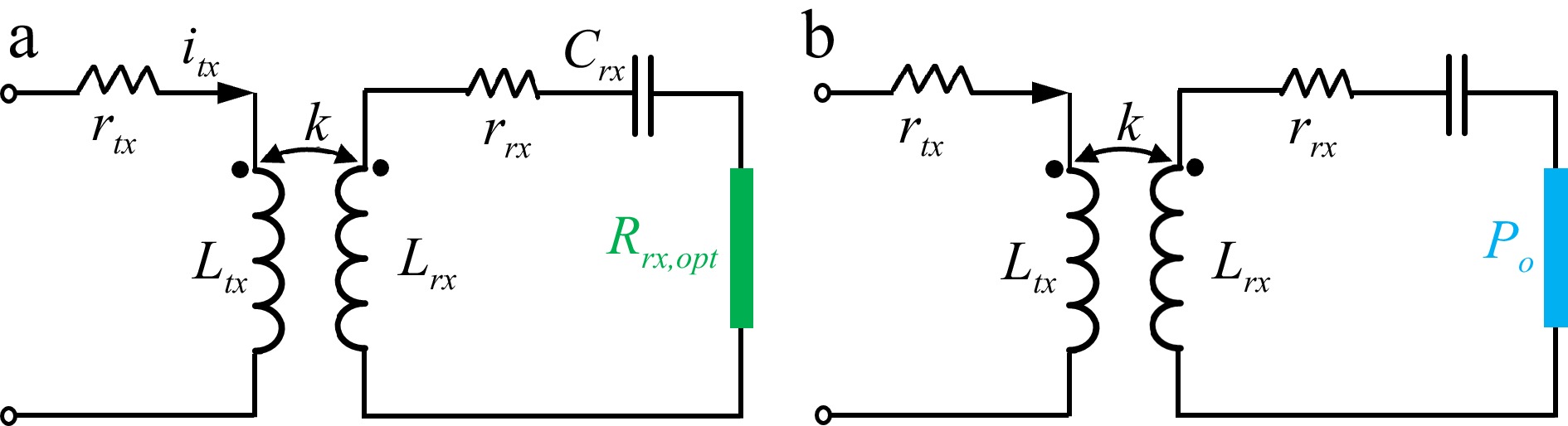
Figure 2.
Equivalent circuit under different control strategies. (a) Optimal load. (b) Optimal excitation.
-
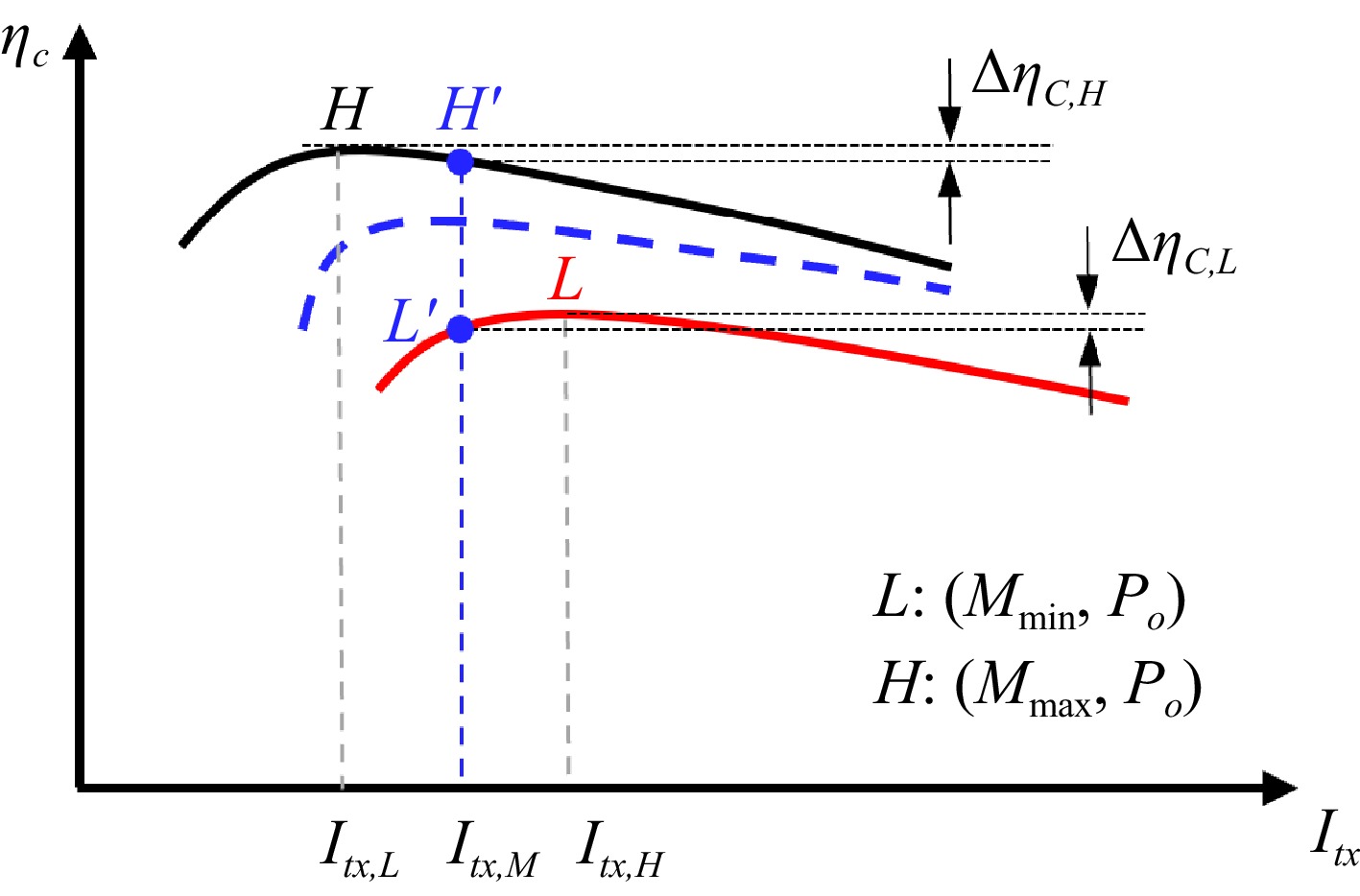
Figure 3.
Coupler efficiency at different
$ k $ $ {I}_{tx} $ -
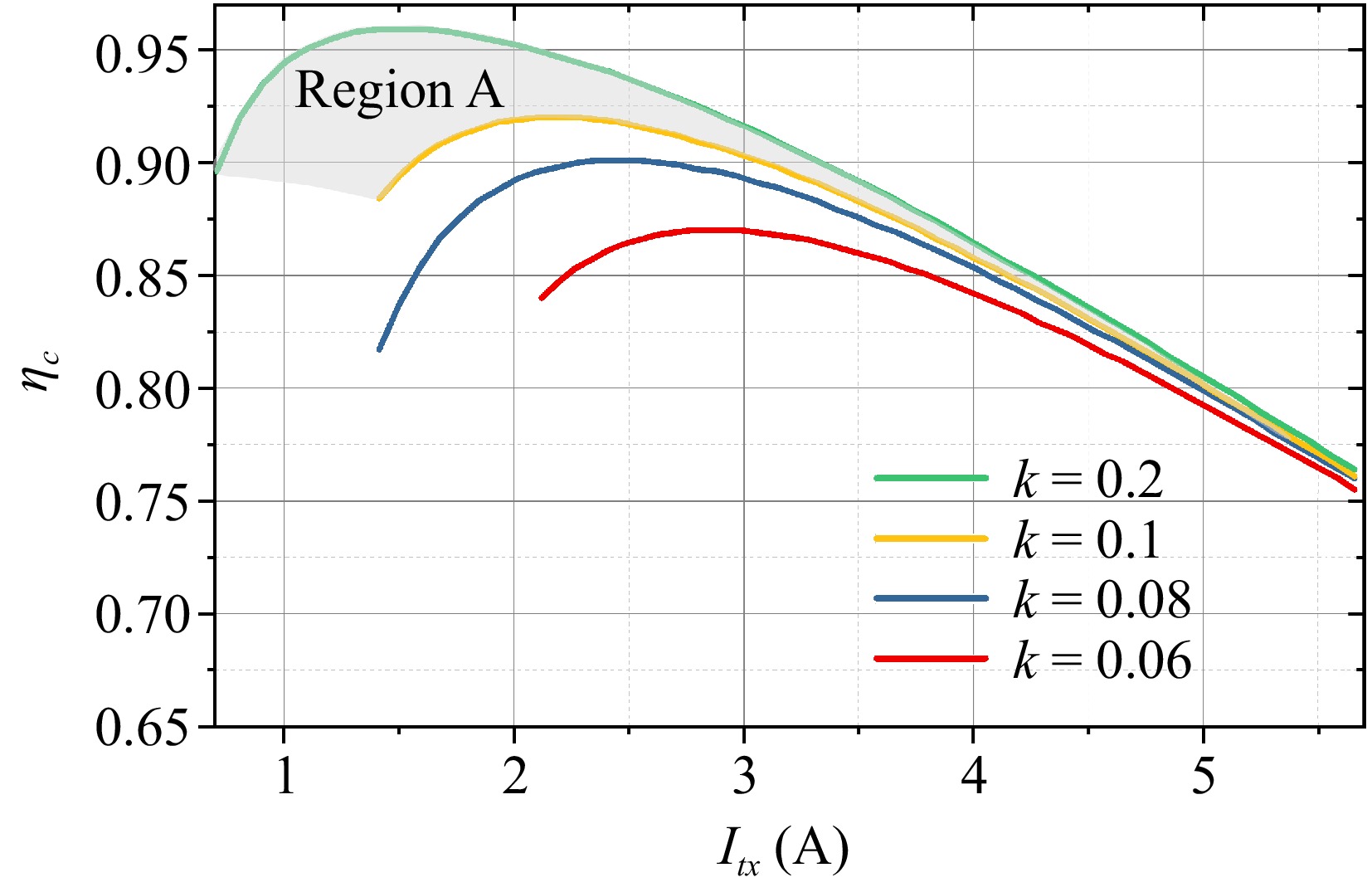
Figure 4.
Efficiency of the 1-RX system under different coupling conditions.
-
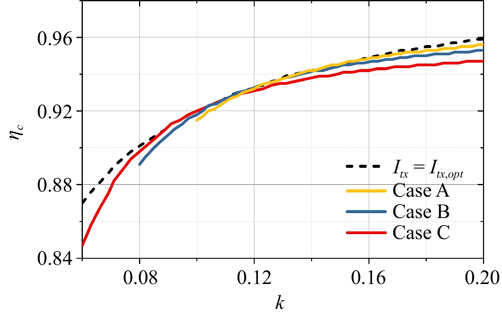
Figure 5.
Efficiency when the coupling range changes.
-
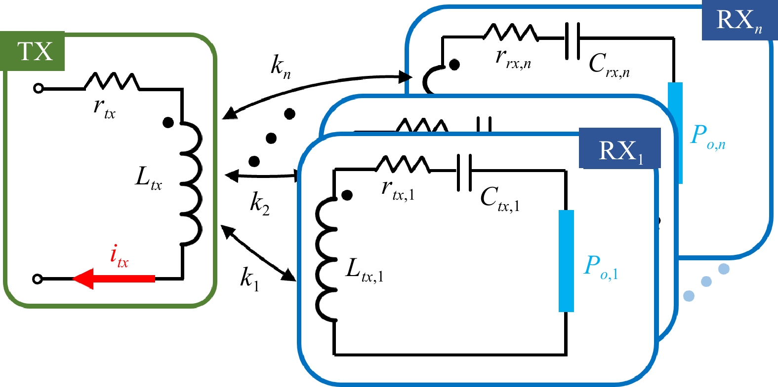
Figure 6.
Simplified circuit model of one-TX n-RX system.
-
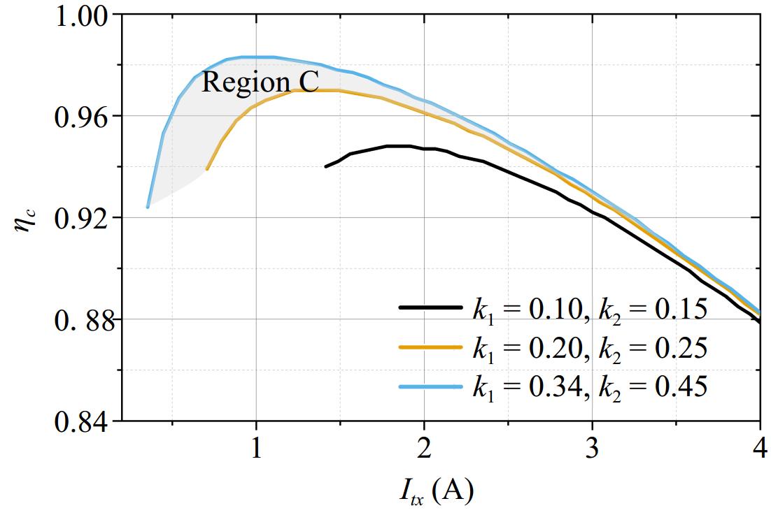
Figure 7.
Coupler efficiency of a 2-RX system under different coupling conditions.
-
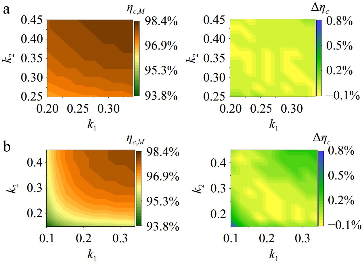
Figure 8.
Efficiency comparison. (a) Case C: ηs,M (left), Δηc (right); (b) Δηc (left), Δηc (right).
-

Figure 9.
Experimental setup.
-
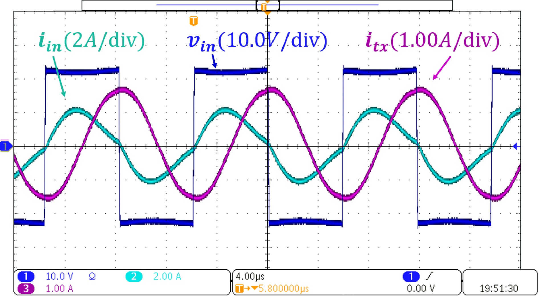
Figure 10.
Experimental waveform.
-
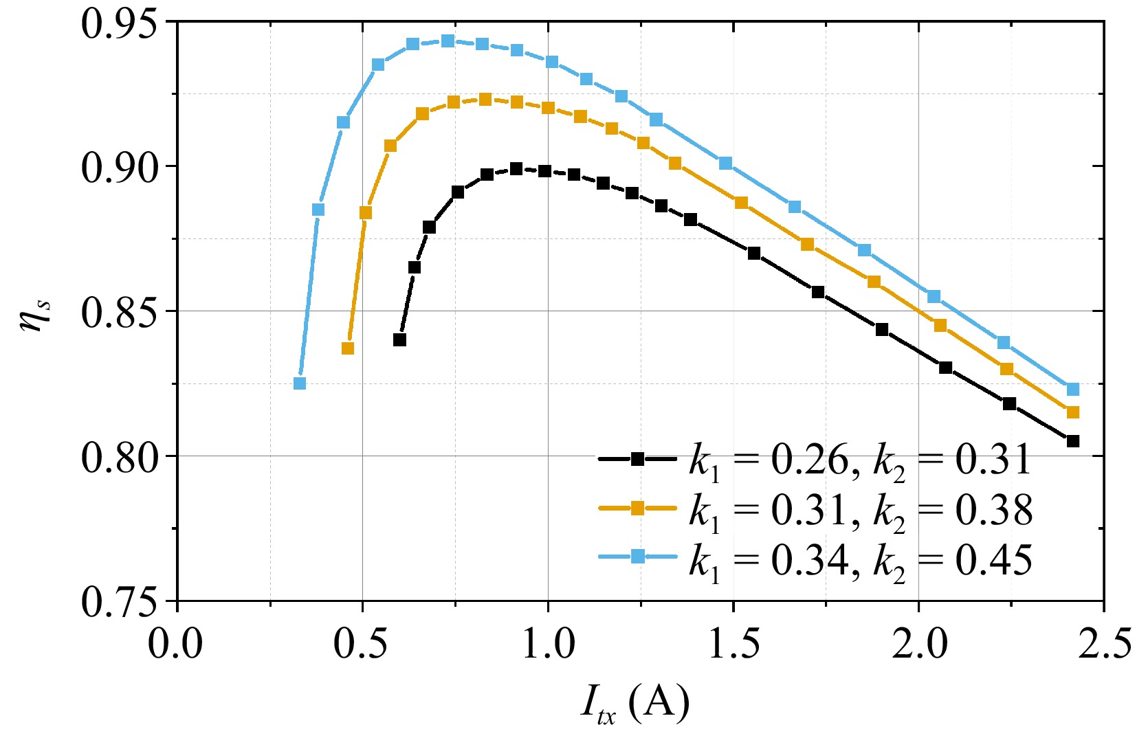
Figure 11.
Efficiency under different coupling conditions.
-
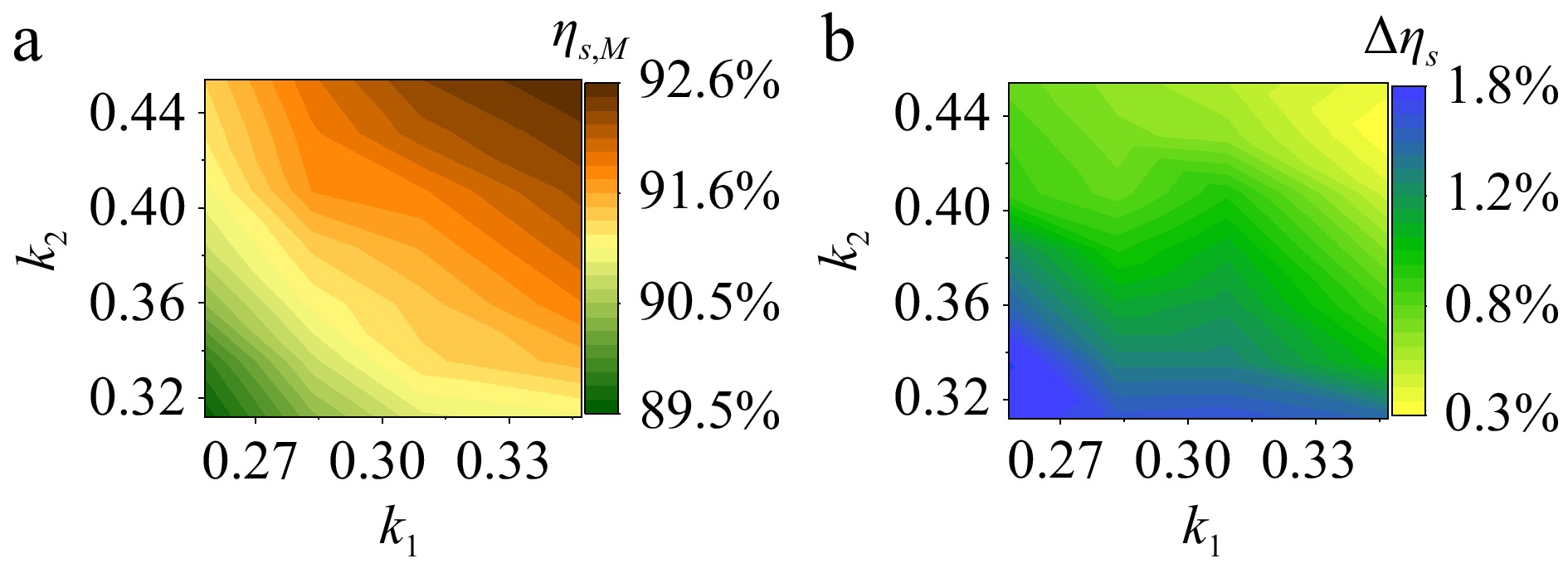
Figure 12.
(a) System efficiency ηs,M. (b) Efficiency drop:
$ \Delta $ -
Symbol Value Symbol Value Symbol Value f 100 kHz Ltx 91.3 μH rtx & rrx 0.195 Ω Lrx,1 22.3 μH rrx,1 0.059 Ω k1 [0.1, 0.34] Lrx,2 26.4 μH rrx,2 0.074 Ω k2 [0.15, 0.45] P1 15 W P2 10 W Table 1.
Parameters of 1TX-2RX IPT system.
Figures
(12)
Tables
(1)