Efficiency control for multi-receiver inductive power transfer systems without knowing realtime coupling

Introduction

In recent years, the widespread use of intelligent mobile terminals has been driving the process of societal intelligence. However, wired charging based on manual connections will severely limit this development^[1]. Inductive power transfer (IPT) has emerged as a promising remedy for charging these intelligent terminals, enabling efficient power transmission from a transmitter (TX) to a receiver (RX). Presently, research focusing on single-TX single-RX IPT systems has achieved considerable maturity. Substantial advancements have been accomplished in coil design, compensation network configuration, output control, efficiency enhancement, and the detection of foreign objects^[2−4]. These developments greatly support the expansion and application of this technology.

Multi-RX charging has emerged as an attractive and challenging area of research. Varied application scenarios present distinct system characteristics, necessitating a focused approach towards system-level design adaptable to diverse power requirements and coupling conditions. In addressing these challenges, extensive discussions have centered around coupler designs, leading to the development of various structures aimed at enhancing and stabilizing the coupling amidst diverse misalignment scenarios^[5,6]. Furthermore, the compensation networks have been recognized as crucial for attaining multiple objectives, including minimizing circulating energy, facilitating soft switching in active circuits, and ensuring output stability amidst load variations^[7]. Notably, beyond passive circuitry, significant progress has been achieved in active circuit designs tailored for multi-RX scenarios^[8,9]. These advancements in coupler and activating circuit designs serve as foundational requisites ensuring the steady-state performance of the system.

A well-performed multi-RX system necessitates an intelligent control methodology to fully exploit its potential benefits. The key control objectives primarily encompass output regulation, power distribution among RXs, and efficiency optimization. For instance, in cases where each RX possesses a specific resonance frequency, employing multiple-frequency excitation allows for independent power control across multiple RXs^[10−12]. The overall efficiency is enhanced in the study by Kim et al.^[13] through the computation of the optimal TX driving current, which heavily relies on the RX-side circuitry and real-time communication. Similarly, a communication-based control strategy has been devised for a system driven by a single Class E inverter, aiding in achieving simultaneous power and efficiency modulation^[14]. Various input modes are formulated in the study of Zhao et al.^[15] to optimize efficiency and cater to diverse power demands. However, these systems predominantly address specific scenarios, failing to comprehensively portray the inherent trade-offs and natural dependencies between achieved performance metrics (such as efficiency and power) and the requisite system complexity (e.g., real-time communication, information sensing, computational burden, and activation of circuits).

This manuscript centers on upholding high efficiency within a single-TX multi-RX system, without knowing real coupling. Employing the single-TX scenario as a case study, the examination delves into the impact of terminal conditions—specifically, the driving current and load—on the resonant tank. This investigation then steers the discourse towards an in-depth analysis of existing approaches aimed at maximizing efficiency at different power. In the absence of real-time coupling knowledge, an optimal current is deduced based on pre-established coupling ranges. As the number of RX grows, the suggested driving logic exhibits considerable scalability and an elevation in system intricacy. The attained efficiency under complete knowledge of all couplings stands as the reference point, only marginally surpassing the efficiency attained through the proposed control strategy.

Single receiver system

System characteristics

The depicted single-TX single-RX IPT system, shown in Fig. 1, encompasses essential components such as the inverter, coupler, compensation unit, rectifier, and load, which collectively elucidate the fundamental control logic. The active circuits, including the inverter, rectifier, and DC/DC converters in both the front-end and post stages, enable input and output modulation for diverse control objectives. Within this system, L_tx and r_tx denote the self-inductance and equivalent series resistance (ESR) of the TX coil, respectively, while L_rx and r_rx represent the self-inductance and ESR of the RX coil. The symbol M signifies the mutual inductance between the coils, while the coefficient k is defined as the coil coupling coefficient: $k=\dfrac{M}{\sqrt{{L}_{tx}{L}_{rx}}}$.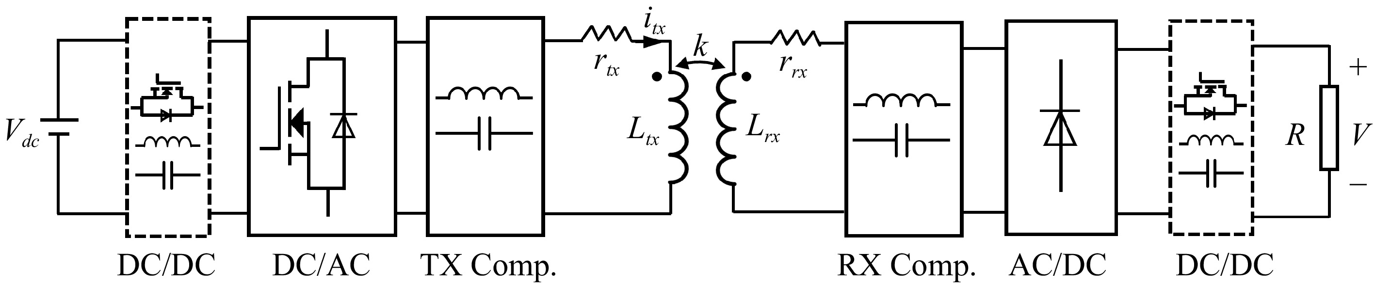

Figure 1.  Configuration of 1TX-1RX system.

DownLoad: Full-Size Img PowerPoint

In Fig. 1, both the TX and RX sides should offer at least two control variables to adjust the output and optimize efficiency indirectly. Typically, these control variables encompass the duty cycle of the DC/DC converter, and the phase shift angle of the inverter, or rectifier. Different combinations of these variables yield various control configurations, as documented in prior studies^[16−18]. Under specific output conditions, such as maintaining a constant voltage (CV), the controllable circuits must satisfy the load's power requirements while ensuring high efficiency throughout the entire system. When dealing with a system incorporating an uncontrollable resonant tank, the diverse configurations and control strategies mentioned earlier can be simplified and clarified through a steady-state analysis of the central resonant tank. This analysis focuses specifically on the integration of compensation and coupler elements and hinges upon terminal conditions—specifically, the input from the TX side and the load output on the RX side.

Despite the existence of various compensations, if assume that losses within the coupler exert a dominant influence on the overall losses, then the efficiency wouldn't be significantly impacted by compensation on the TX side. Consequently, this study is aimed at investigating the passive network depicted in Fig. 2, where TX compensation is disregarded, and a straightforward series compensation is implemented on the RX side. In this setup, C_rx denotes the series compensating capacitor, fulfilling the condition 1/(ωC_rx) = ωL_rx, while i_tx represents the input current to the TX coil.

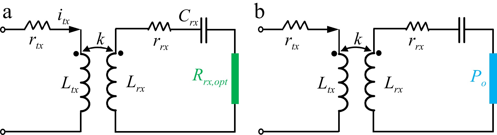
Figure 2.  Equivalent circuit under different control strategies. (a) Optimal load. (b) Optimal excitation.

DownLoad: Full-Size Img PowerPoint

In terms of the load viewpoint, controllable systems can be classified into two distinct types. The first type involves manipulating the RX-side circuitry to attain the optimal load while simultaneously adjusting the TX-side excitation to fulfill the output power requirements, as illustrated in Fig. 2a. In this arrangement, the rectifier and its subsequent circuit components are treated as a load resistance R_rx,opt when aiming for maximum coupler efficiency. The RX's output power during resonance is expressed as:

The optimal load resistance R_rx,opt for efficiency maximization has been well studied and derived as:

By solving Eqns (1) and (2) concurrently, it gives the root mean square (RMS) value of the necessary input current under the optimal condition, expressed as follows:

The efficiency of the coupler is:

which is loading and coupling dependent.

The second type of system aims to provide optimal driving current to maximize efficiency, and its load model is illustrated in Fig. 2b. In this setup, the RX-side circuit maintains the desired output characteristics, such as a constant voltage (CV), while satisfying specific power requirements P_o through RX-side control. Simultaneously, the TX-side circuit adjusts the input excitation to enhance efficiency. Despite the differing control methodologies between these two types, the eventual steady-state effects remain consistent. The primary difference lies in the approaches used to achieve this optimal state, involving distinctions in the activation of circuits, communication protocols, and the requisite information, particularly the coupling.

In Fig. 2b, maximizing efficiency is equivalent to minimizing losses for a target power. The power loss is expressed as:

The optimal excitation at this point can be determined by solving the equation $\dfrac{d{P}_{\mathrm{l}\mathrm{o}\mathrm{s}\mathrm{s}}}{d{I}_{\mathrm{t}\mathrm{x}}}=0$, yielding the coil's input current excitation I_tx,iopt, which would further determine the corresponding optimum efficiency η_c,iopt. Based on derivation, it would find I_tx,iopt = I_tx,ropt and η_c,iopt = η_c,ropt. The fact that both types of systems share the same excitation in the steady state indicates that, despite different control methods and transient processes, the systems reach identical stable states, i.e., there exists only one global maximum efficiency point. If R_rx,opt $\mathrm \gg$ r_rx, the losses on the TX and RX coils are equal and can be expressed as:

It physically means the optimal efficiency indicates a loss balance condition.

By employing optimal load control as illustrated in Fig. 2a, achieving R_rx,opt demands coupling information for the RX, while the TX relies on receiving feedback (usually via wireless communication) from the RX to regulate power^[19]. Conversely, using the second approach depicted in Fig. 2b allows independent regulation of the RX through a linear controller. In the absence of communication, the TX must resort to either a non-linear tracking algorithm or a sensing-based coupling estimation approach to provide the necessary optimal driving current^[20]. Consequently, a noticeable trade-off emerges involving the communication requirement, controller type, and sensing necessity.

Excitation current based on coupling range

This paper presents a simplified excitation control approach based on the coupling range. The proposed method simplifies the control process by requiring determination of the coupling coefficient range during the coupler design phase. Following implementation, the system operates autonomously, obviating the necessity for real-time coupling estimation or nonlinear tracking algorithms. The core operational principle is demonstrated initially in a straightforward single-RX scenario, subsequently extending its applicability to a more intricate multi-RX scenarios.

In a single-RX system, ensuring sufficient coupling generally requires the RX to be charged within a specified charging area. In such instances, the range of coupling coefficient variations is limited and becomes known upon the fabrication of the coupler. The controllable circuit on the RX side can uphold a constant voltage output (fulfilling the load power requirements), while the TX side employs a real-coupling-independent control. The excitation current is determined by the range of coupling variations.

Figure 3 illustrates the efficiency curve of the coupler, demonstrating variations in input currents while regulating the RX side to achieve the target power. Within the graph, M_min signifies the minimum mutual inductance, M_max signifies the maximum mutual inductance, P_o represents the output power, and the upper and lower boundaries are established by the coupling range. The solid black line represents the system response at maximum coupling, while the solid red line represents the system response at minimum coupling. Within the determined coupling range, the actual response curve of the system is denoted by the dashed blue line. Given offset conditions, the blue line remains constrained within the upper and lower boundaries.

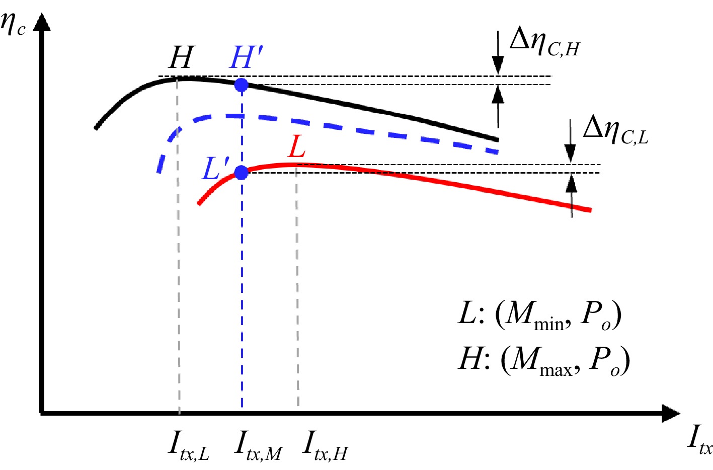
Figure 3.  Coupler efficiency at different $k$ and ${I}_{tx}$.

DownLoad: Full-Size Img PowerPoint

In Fig. 3, L denotes the optimal efficiency point when the coupling is at its minimum. According to Eqn (3), this point is associated with an optimal input excitation, I_tx,L, given by:

Here, H corresponds to the optimal point when the coupling is at its maximum, associated with an optimal excitation, I_tx,H, given by:

If employing the non-linear perturbation observation method, the system requires continuous tracking of the optimal excitation between I_tx,L and I_tx,H^[21]. Despite the absence of direct communication between the TX and RX sides, disturbances on the TX side can affect the stability of the RX side output. In scenarios without non-linear tracking, estimating the coupling based on TX side information becomes necessary to maintain the coupling-dependent optimal current^[20].

Within the specified coupling range, this paper proposes a strategy that utilizes the average of I_tx,L and I_tx,H as the driving current, denoted as:

The median current value, I_tx,M, is influenced by coil parameters, load power, and the coupling range. When the real coupling is M_min, the operating point becomes L' using I_tx,M as the driving current. The efficiency difference between L' and L is Δη_C,L. Conversely, at maximum coupling, the operating point is H', and the efficiency difference between H' and H is Δη_C,H. Δη_C,L and Δη_C,H depict the trade-off incurred by using the real-coupling-independent I_tx,M.

The proposed excitation control strategy eliminates the necessity for real-time tracking of the highest efficiency point and instead maintains operation at a compromise point. At this juncture, the TX side losses stabilize at ${I}_{tx,M}^{2}\cdot {r}_{tx}$, and different couplings determine varying currents on the RX-side coil. When the current on the RX-side coil reaches a certain value such that the losses at both ends of the coil become equal, i.e., ${I}_{tx,M}^{2}\cdot {r}_{tx}={I}_{rx}^{2}\cdot {r}_{rx}$, the system attains its actual maximum efficiency point.

Influence of coupling range

To provide a quantitative verification and study the impact of the coupling range, a simulation is employed for further elucidation of the qualitative analysis. The simulation utilizes the following parameters: f = 100 kHz, L_tx = 90 μH, L_rx = 75 μH, r_tx = 0.192 Ω (Q_tx = 250), r_rx = 0.174 Ω (Q_rx = 230), and P_o = 20 W. As the coupling varies, the coupler efficiency changes with the input excitation, as depicted in Fig. 4. Region A delineates the operational area when k ranges within [0.1,0.2]. The simulation results indicate that with an increase in k, the corresponding optimal excitation current decreases.

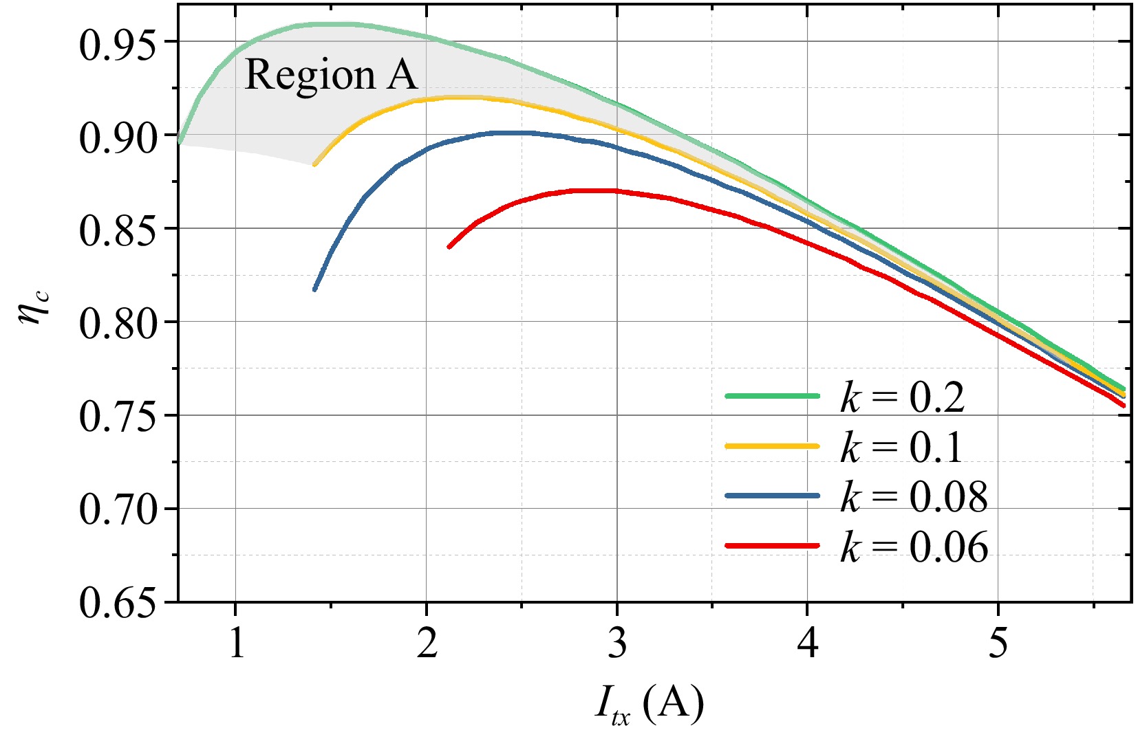
Figure 4.  Efficiency of the 1-RX system under different coupling conditions.

DownLoad: Full-Size Img PowerPoint

If the driving current is controlled to be the optimal value, i.e., I_tx = I_tx,opt, the efficiency is depicted by the black dashed line in Fig. 5, which connects all peak points of Fig. 4. This reference curve serves as the basis for analyzing the influence when I_tx changes to I_tx,M. For instance, considering k $\in$ [0.1, 0.2], the efficiency achieved by I_tx,M—calculated using Eqns (7), (8), and (9)—is represented as case A (yellow solid line) in Fig. 5. It marginally falls below the reference curve, with a maximum drop of 0.5%. Expanding the coupling range to k $\in$ [0.08, 0.2], corresponding to the region between the green and blue solid lines of Fig. 4, yields the efficiency achieved by I_tx,M represented as case B in Fig. 5, exhibiting a maximum drop of 1%. When k $\in$ [0.06, 0.2], as demonstrated in case C, it results in a maximum 2% efficiency drop. These simulation outcomes indicate that adopting I_tx,M based on the coupling range demonstrates efficiency performance close to real-time tracking of the optimal excitation, showcasing favorable system characteristics.

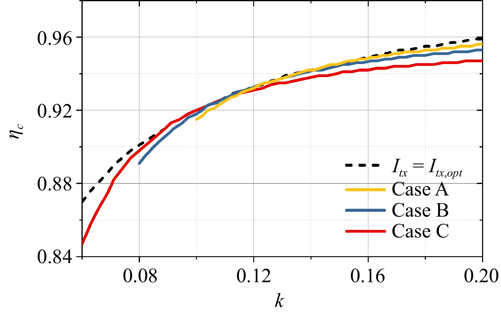
Figure 5.  Efficiency when the coupling range changes.

DownLoad: Full-Size Img PowerPoint

Multi-RX system

System characteristic and optimal driving current

Figure 6 illustrates a single-TX n-RX system. L_rx,j and r_rx,j denote the self-inductance and ESR of the j-th RX coil. k_j is the coupling coefficient between the TX and the j-th RX, satisfying: ${k}_{j}={M}_{j}/\sqrt{{L}_{tx}{L}_{rx,j}}$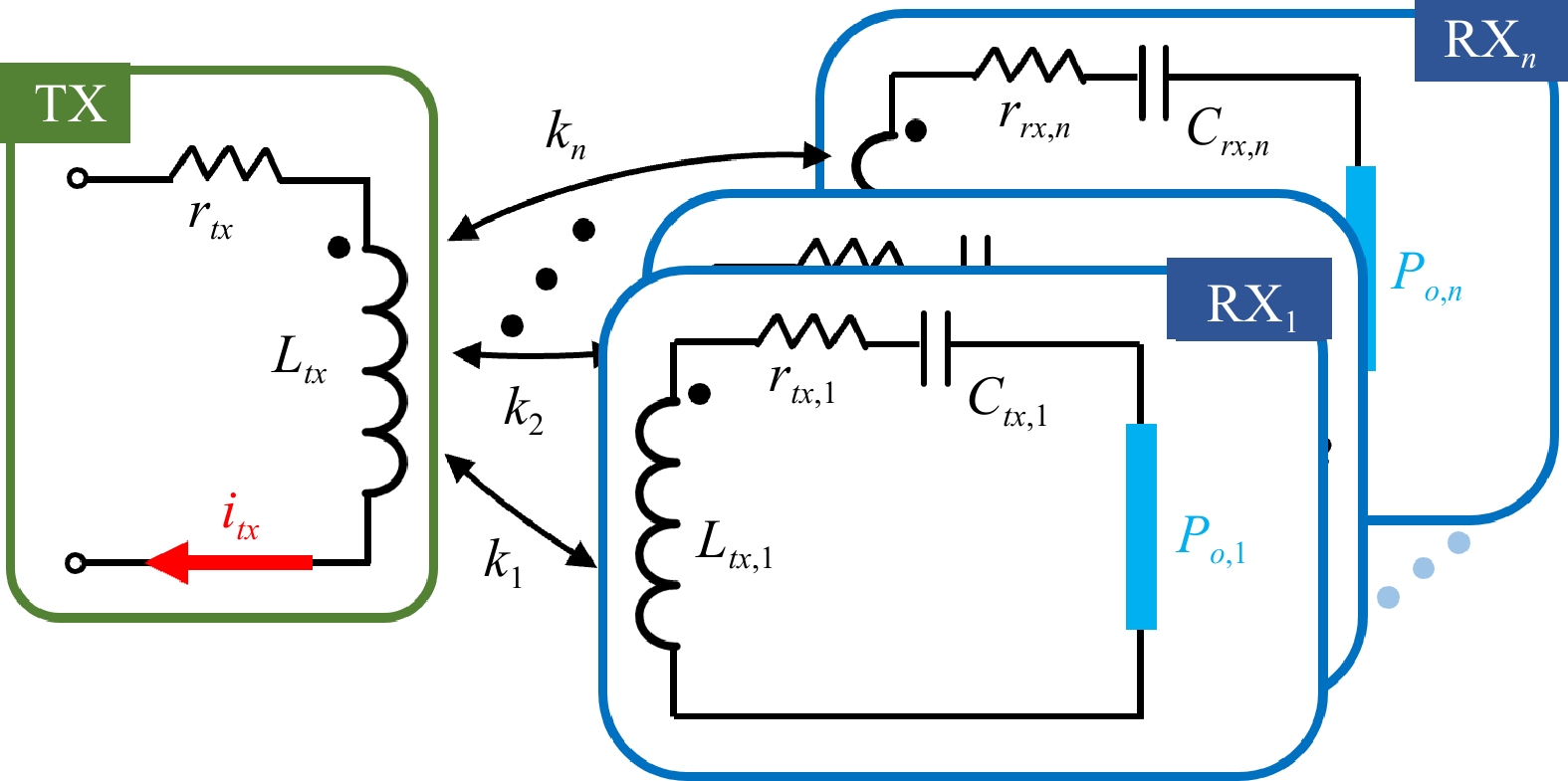. C_rx,j is the series compensation capacitor, and R_rx,j is the equivalent AC load resistance. The resonance on the RX side satisfies the condition: ωL_rx,j − 1/(ωC_rx,j) = 0. In scenarios where charging occurs in a flat plane, having multiple RXs positioned over the TX charging area can induce cross-coupling between the RXs. Since the RX coil is enclosed within the device, the minimum coil clearance between adjacent devices becomes a variable during the design phase. Adequate clearance between coils is essential to minimize cross-coupling effects. Consequently, the analysis conducted above assumes a model where the RX cross-coupling is not considered.

Figure 6.  Simplified circuit model of one-TX n-RX system.

DownLoad: Full-Size Img PowerPoint

Similar to the single RX scenario depicted in Fig. 2, when employing different control logics in RXs, it becomes essential to individually examine the optimal conditions achieved. In scenarios where the system offers multiple control options, adjusting the load resistance at each RX becomes crucial to maximize coupler efficiency. As outlined in the study by Fu et al.^[22] , the necessary load resistance values and their respective efficiencies are:

In contrast to the single-RX system, the aforementioned multi-RX system possesses n power outputs and n optimal load resistance values. It offers n + 1 degrees of freedom for control, provided by the TX and RX sides (n on the RX side, 1 on the TX side). To achieve global optimal efficiency, i.e., satisfy Eqn (11), each load should adhere to the optimal load condition, i.e., Eqn (10), through its respective control circuit. In this scenario, the power distribution among the loads is constrained to follow the following proportions:

There are no degrees of freedom available for power regulation. Therefore, the control logic of Fig. 2a cannot be extended to a multi-RX scenario.

When the RX-side circuit is dedicated to maintaining a constant voltage, the excitation current on the TX side becomes pivotal in enhancing the system's efficiency. This reflects the optimal excitation control employed in a scenario featuring a single TX and a single RX. In this context, maximizing the system's efficiency can be reformulated as a problem centered on minimizing losses while adhering to equality constraints, as articulated below:

The method for solving such an optimization problem involves the Lagrange multiplier method. Equation (14) represents the Lagrangian, where L is the Lagrange function, and λ_i is the Lagrange multiplier.

If ${R}_{rx,opt}\gg {r}_{rx}$, by solving $\dfrac{\partial L}{\partial {I}_{tx}}=0$ and $\dfrac{\partial L}{\partial {\lambda }_{j}}=0$, the optimal input excitation current I_tx, of the system under known coupling coefficients, which maximizes system efficiency, can be obtained as follows:

Substituting Eqn (15) into the efficiency expression yields:

At this point, the coupler achieves an efficiency η_c,iopt while facing power constraints on the RX side, rather than the globally optimal efficiency η_c,ropt obtained without power constraints, expresses the system efficiency when operating at the global optimum, representing the theoretical efficiency limit of the system. Therefore, η_c,iopt ≤ η_c,ropt, signifying that under the control strategy of optimal excitation, the efficiency is always lower than the efficiency under optimal load conditions. The losses on the TX and RX sides at this point are given by:

This conclusion indicates that under optimal excitation, the coil conduction losses on the TX side and RX side are equal, consistent with the characteristics of a single-RX system [refer to Eqn (5)].

From the above analysis, it can be concluded that for a general multi-RX system with different RX coils, various couplings, and distinct power requirements, when the coil parameters and output power are determined, the coupler efficiency depends solely on the coupling and the input excitation I_tx. This characteristic is akin to the single-RX case. Despite the increase in the number of outputs, the control freedom of TX remains unchanged. The upper and lower boundaries of the efficiency curve are still determined by the coupling variation range. Therefore, the efficiency curve shown in Fig. 4 is still applicable to a multi-RX system. The red solid line represents the efficiency curve when the coupling between the TX and all RXs is minimized (i.e., M_j = M_min). At this point, the current at the efficiency peak L is given by:

The black solid line represents the efficiency curve when the coupling between the TX and all RXs is maximized (i.e., M_j = M_max). The current at the corresponding efficiency peak is given by the following:

It is possible to adopt the average current, which mirrors the approach used in the single-RX system, i.e.,

which is also influenced by coil parameters, load power, and the coupling range. Given the known coupling range, the input excitation is determined without the need for real-time coupling information. When using the proposed excitation, the TX coil loss is ${P}_{loss,tx}={I}_{tx,M}^{2}{R}_{tx}$, while the RX-side losses vary with the coupling. When the coupling changes to the condition given by Eqn (17), where the sum of RX-side losses equals the TX side losses, the system reaches its optimal efficiency state, calculated as Eqn (16).

In a single-RX system, the TX side must obtain specific coupling and load information through communication or detection means and then calculate the optimal excitation. Similarly, in a multi-RXs system, if coupling estimation or similar methods are employed, the difficulty of estimating information and the circuit cost will increase dramatically due to the addition of RX devices. Therefore, the proposed driving strategy would show great scalability and is particularly advantageous in multi-RX systems.

Influence of coupling range

Taking the example of a dual-RX system to study the influence of coupling, Table 1 shows the simulation parameters. The coupling range is k₁ $\in$ [0.1, 0.34] for RX1, and k₂ $\in$ [0.15, 0.45] for RX2. In Fig. 7, when meeting the power demand, the coupler efficiency changes with input excitation, and different colors represent different coupling conditions. The blue line represents the coil efficiency change curve when the coupling is strongest (k₁ = 0.2, k₂ = 0.25), the orange curve represents an intermediate state (k₁ = 0.34, k₂ = 0.45), and the black solid line is used to represent the weakest coupling (k₁ = 0.1, k₂ = 0.15). Similar to Fig. 4, stronger coupling leads to a smaller optimal excitation current and higher efficiency. Additionally, the power level and coil parameters also influence the shape and position of the efficiency curve.

Table 1.  Parameters of 1TX-2RX IPT system.

Symbol	Value		Symbol	Value		Symbol	Value
f	100 kHz		Ltx	91.3 μH		rtx & rrx	0.195 Ω
Lrx,1	22.3 μH		rrx,1	0.059 Ω		k1	[0.1, 0.34]
Lrx,2	26.4 μH		rrx,2	0.074 Ω		k2	[0.15, 0.45]
P1	15 W		P2	10 W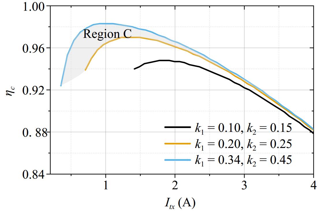

 | Show Table

DownLoad: CSV

Figure 7.  Coupler efficiency of a 2-RX system under different coupling conditions.

DownLoad: Full-Size Img PowerPoint

Analogous to the single-RX system, for certain spatial offsets in practical applications, real-coupling-independent I_tx,M is calculated by simultaneously solving Eqns (18), (19), and (20). Therefore, when I_tx,M and I_tx,opt are used, the efficiency difference can explain the high-efficiency operation.

The coupling range denoted by region C of Fig. 7 means k₁ $\in$ [0.2, 0.34] and k₂ $\in$ [0.25, 0.45]. It is defined as Case C, and the corresponding simulation results are shown in Fig. 8a. The left graph illustrates the coupler efficiency η_c,M under excitation I_tx,M, while the right graph displays the efficiency difference Δη_c between the maximum coil efficiency η_c,iopt (using I_tx,opt) and η_c,M (using I_tx,M). Within the coupling range, the efficiency difference is less than 0.2%. As shown in Fig. 8b, with a further expansion of the coupling range in Case D (k₁ $\in$ [0.1, 0.34], k₂ $\in$ [0.15, 0.45]), the maximum efficiency drop is 0.8%. From these examples, it is evident that adopting the proposed current would maintain relatively high coupler efficiency without dramatically increasing the requirement of real-time coupling information.

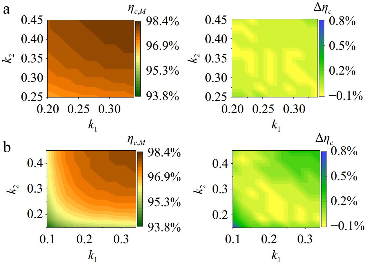
Figure 8.  Efficiency comparison. (a) Case C: η_s,M (left), Δη_c (right); (b) Δη_c (left), Δη_c (right).

DownLoad: Full-Size Img PowerPoint

Experimental verification

An experimental platform was implemented using a single-TX dual-RX system to validate the theoretical conclusion. As illustrated in Fig. 9 the setup includes a DC source, a full-bridge inverter, a large square TX coil, two small RX coils (rectangular RX1 and square RX2), rectifiers, and loads. The TX side employs an LCC compensation structure, while the RX sides utilize series compensation. This compensation is convenient to use the DC input voltage for the TX coil current control due to the clamping effect. The coil parameters are provided in Table 1, and the compensation parameters are as follows: L_t = 32 μH, C_t = 110 nF, C_tx = 57 nF, C_rx1 = 227 nF, C_rx2 = 132.8 nF. The charging powers for the two loads are P₁ = 10 W and P₂ = 15 W.

Figure 9.  Experimental setup.

DownLoad: Full-Size Img PowerPoint

When two RXs are placed within a specific charging area in Fig. 9 (i.e., not moving outside the TX), the coupling variation ranges are measured as k₁ $\in$ [0.2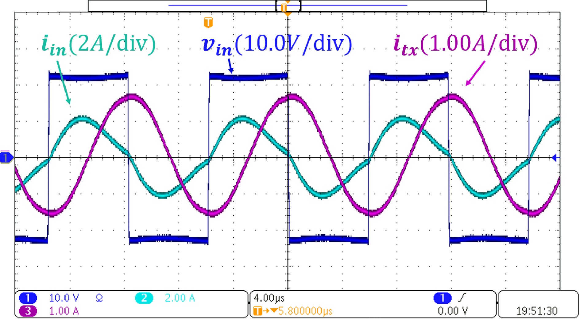6, 0.34] and k₂ $\in$ [0.31, 0.45]. Using the driving current Eqn (20), with an effective value of I_tx,M = 1.151 A, a corresponding DC voltage of V_dc = 23 V is provided. Note that the coil current is clamped by the input DC voltage in LCC compensation. Within the mentioned coupling variation range and power demands, the experimental waveforms of inverter output voltage v_in, input current i_in, and TX coil input current i_tx are depicted in Fig. 10. When employing I_tx,M, v_in, and i_tx remain constant, while i_in exhibits slight fluctuations under coupling variation.

Figure 10.  Experimental waveform.

DownLoad: Full-Size Img PowerPoint

The efficiency analysis in the preceding section exclusively concentrates on the coupler itself, but the efficiency is also influenced by compensations, inverters, and rectifiers. And the characteristic traits of the efficiency curve primarily stem from the attributes of the coupler. Past studies have emphasized that a precise analysis of system efficiency necessitates the consideration of all loss models. However, when optimizing efficiency, the control mechanisms often resort to simplified analyses to deduce the terminal requisites for the resonant tank. Hence, in the ensuing analysis, a comprehensive system-level evaluation could be undertaken to yield results akin to those illustrated in Figs 7 and 8.

Similar to the AC simulation in Fig. 7, the influence of the coupling could be studied in a complete DC to DC system. The overall efficiency η_s is measured by sweeping the input current as shown in Fig. 11. An optimal current exists, and it is still valid to have a conclusion that a stronger coupling leads to a lower optimal current.

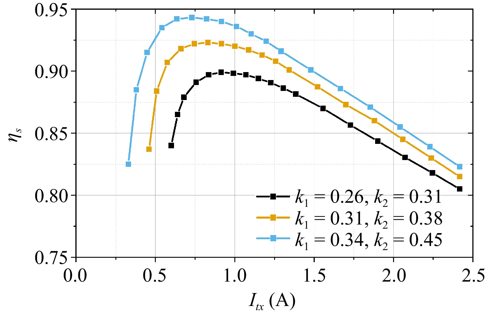
Figure 11.  Efficiency under different coupling conditions.

DownLoad: Full-Size Img PowerPoint

When employing I_tx,M, as illustrated in Fig. 10, and moving two RX coils to change their coupling, the input and output power were measured using a power analyzer. The system efficiency η_s,M is then obtained in Fig. 12a, which changes from 89.5% to 92.6%. Simultaneously, the optimal efficiency values η_c,sopt (obtained by sweeping the input current) under different couplings are measured and compared with η_s,M. The difference is illustrated in Fig. 12b. At higher coupling, η_s,M is closer to η_s,opt, differing by only 0.4%. As the coupling weakens, the efficiency difference gradually increases, reaching a maximum of 1.7%. The proposed control can maintain high-efficiency operations without the need for coupling estimation.

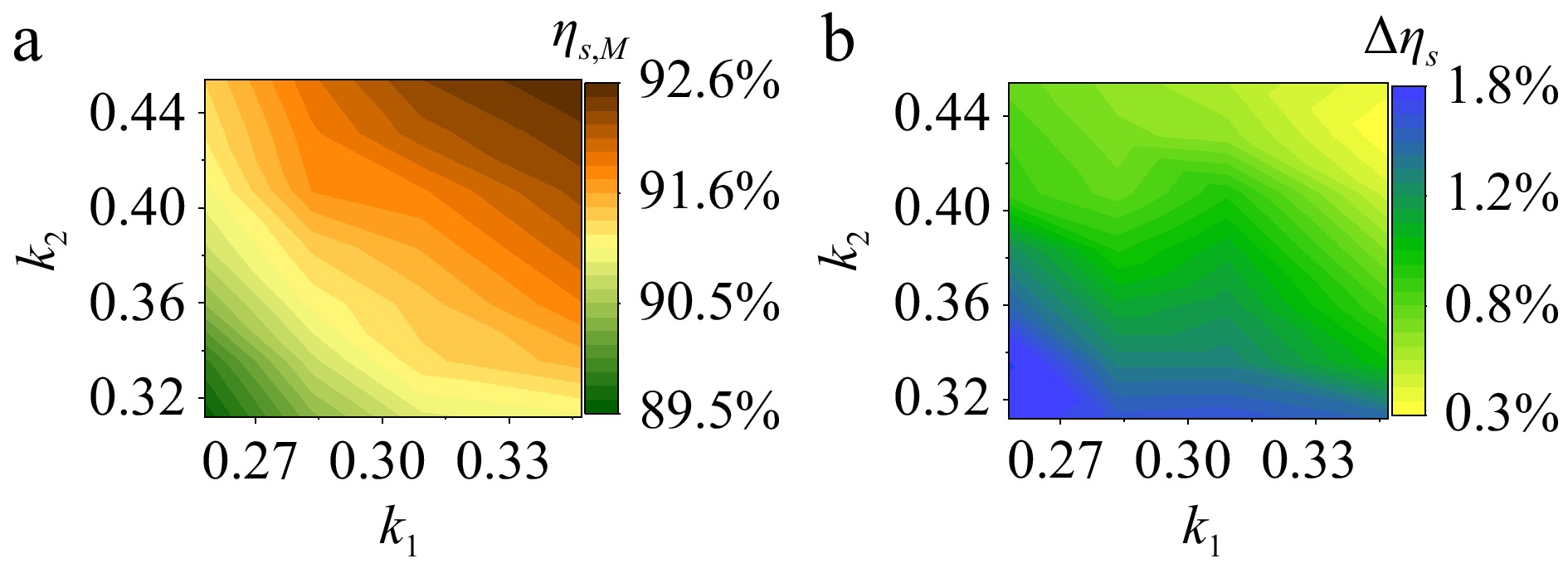
Figure 12.  (a) System efficiency η_s,M. (b) Efficiency drop: $\Delta$η_s = η_s,opt − η_s,M.

DownLoad: Full-Size Img PowerPoint

The similar trends in simulation and experiment indicate that the differences in efficiency are mainly attributed to the losses in the active circuits (inverter and rectifier) and conductor losses. The AC analysis in the previous sections would be used to guide the current control in a complete DC-to-DC system. The experimental results demonstrate that the proposed excitation based on the coupling range maintains a certain level of high efficiency, with stable input and simple control strategies.

Conclusions

This paper proposes a simple driving logic to dramatically improve the scalability of a general single-TX multi-RX IPT system. The high-efficiency operation is achieved without knowing the real coupling and does not suffer from the coupling variation issue. Using the one-RX example, the coupler analysis unified the understanding of optimal conditions, which serves as the reference to justify the benefit of the proposed excitation. The same control logic is then extended to a general multi-RX case based on the derivation of optimal conditions. The claimed benefit is finally verified in a complete two-RX system.

Acknowledgments

This work was supported by National Natural Science Foundation of China (Grant No. 52477013).