Back Article

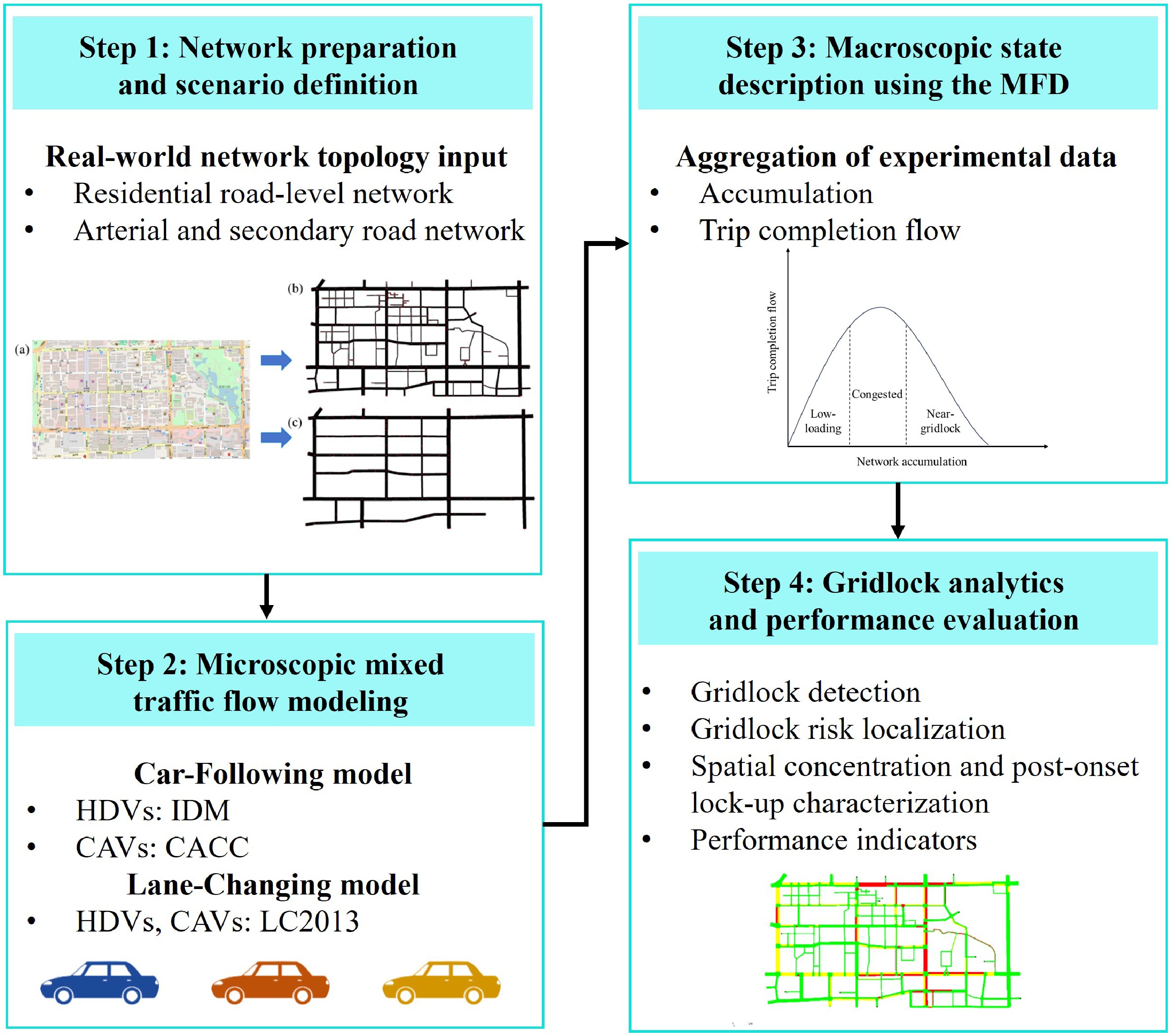
Figure 1. 

Overall analytical framework.

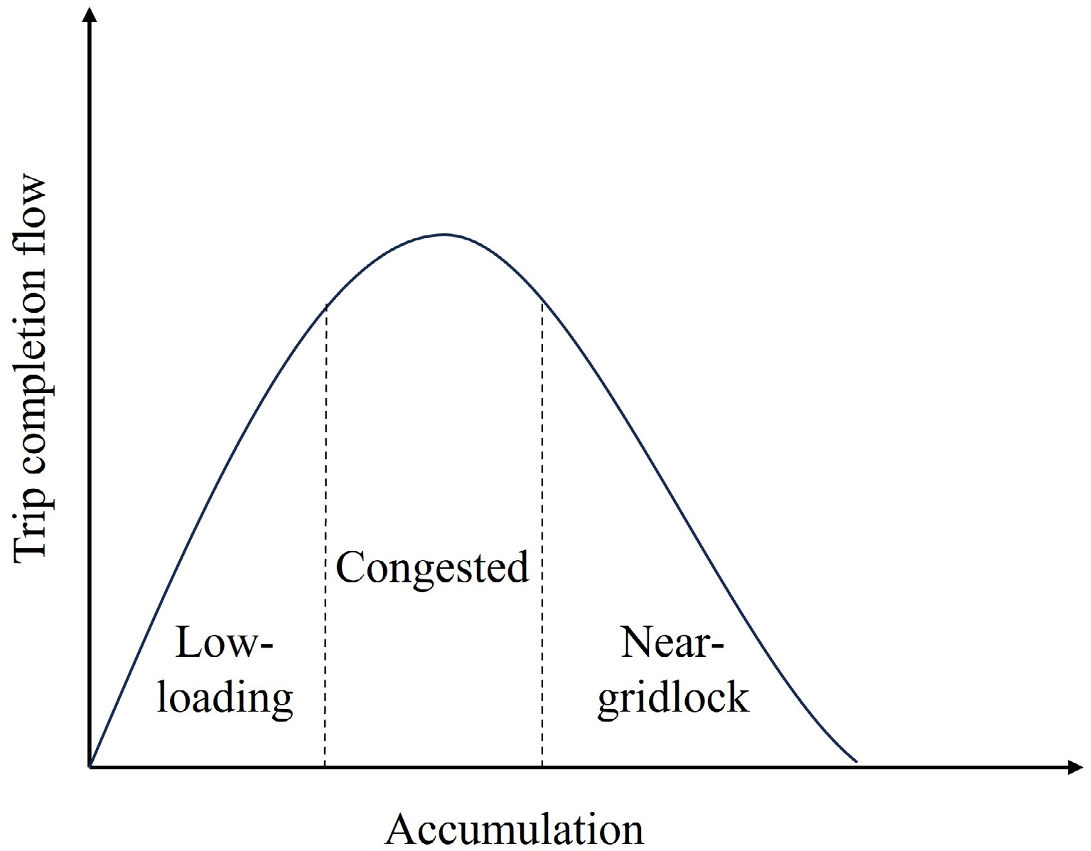
Figure 2. 

Macroscopic fundamental diagram.

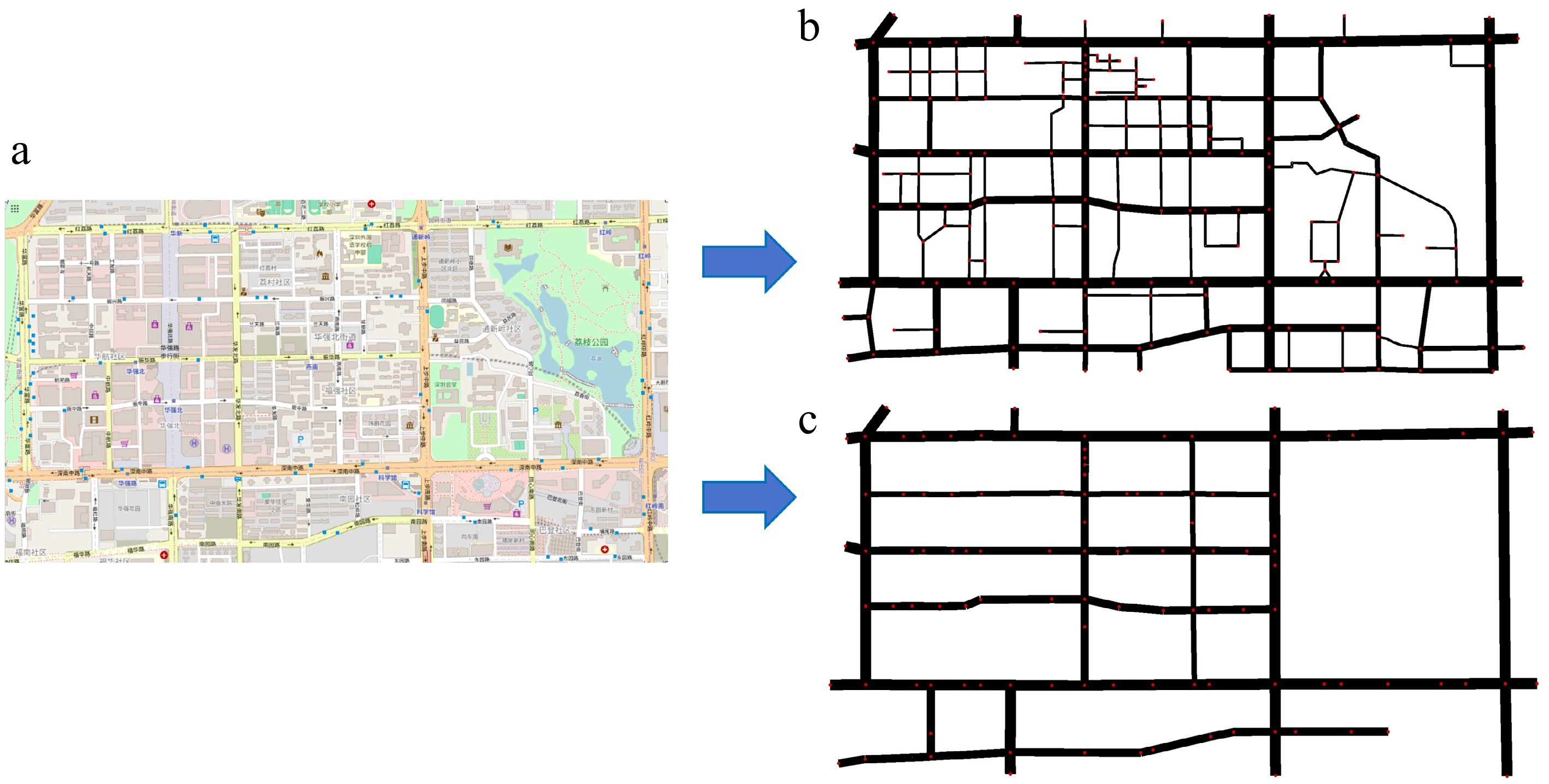
Figure 3. 

Simulation network. (a) The real-world network map, (b) Network 1, and (c) Network 2.

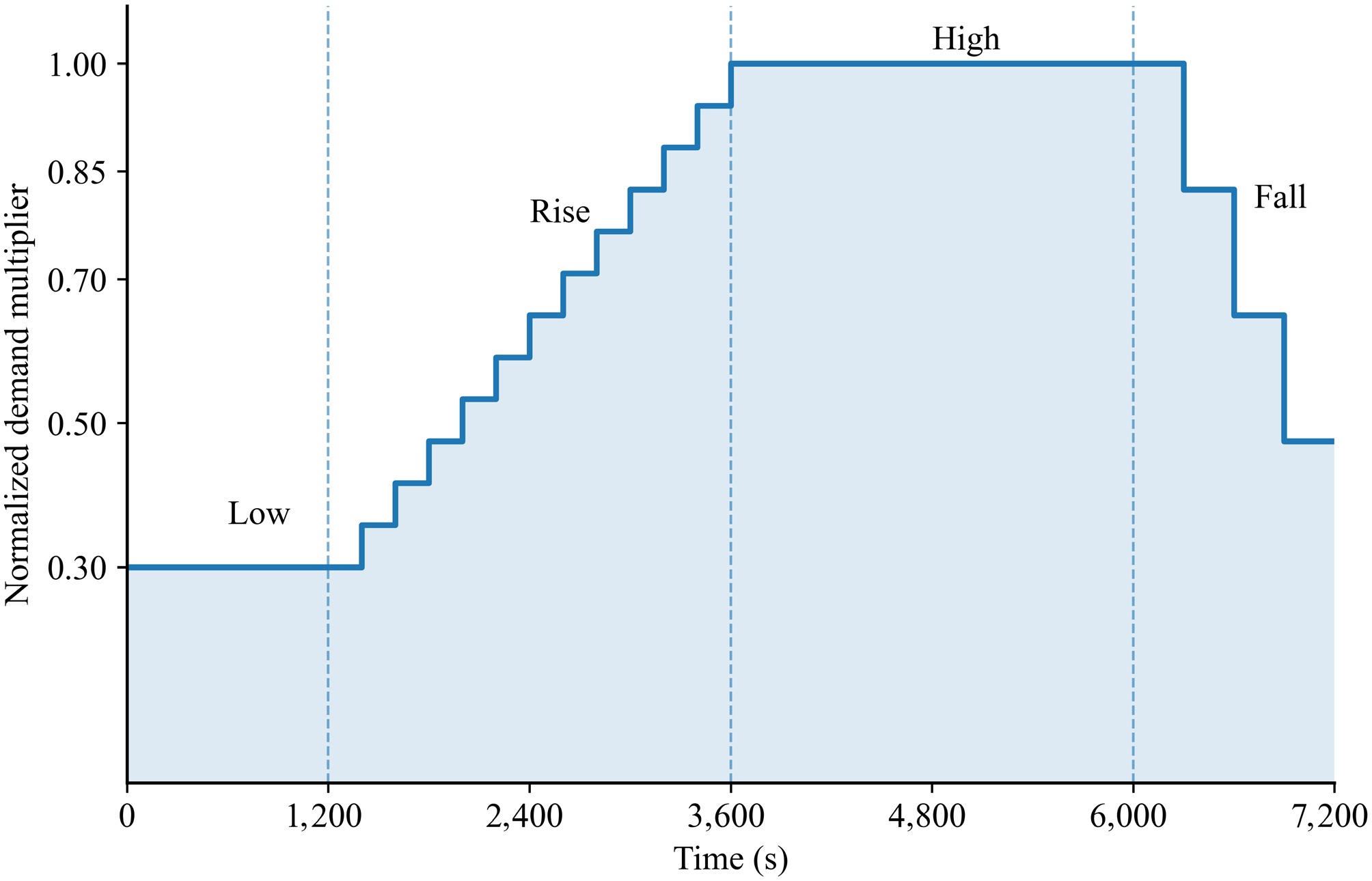
Figure 4. 

Demand-loading scheme.

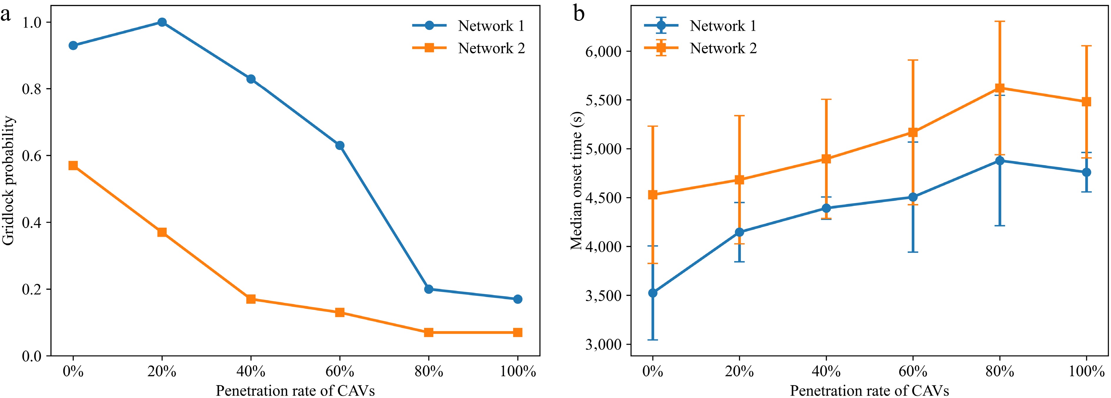
Figure 5. 

Gridlock probability and onset-time distribution under different CAV penetration rates. (a) Gridlock probability. (b) Median onset time.

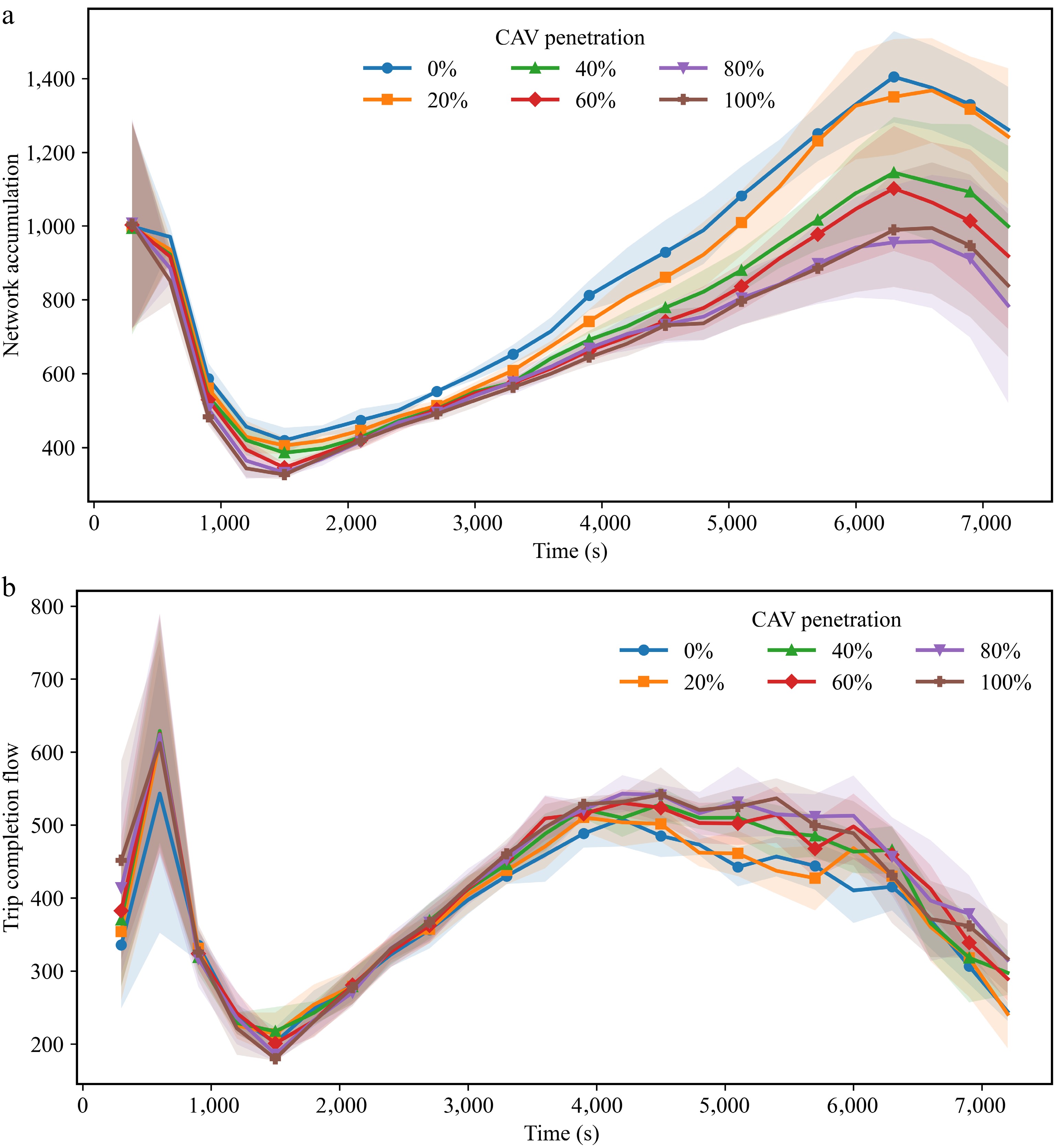
Figure 6. 

Temporal evolution of network accumulation and trip completion flow under different CAV penetration rates. (a) Temporal evolution of network accumulation. (b) Temporal evolution of trip completion flows.

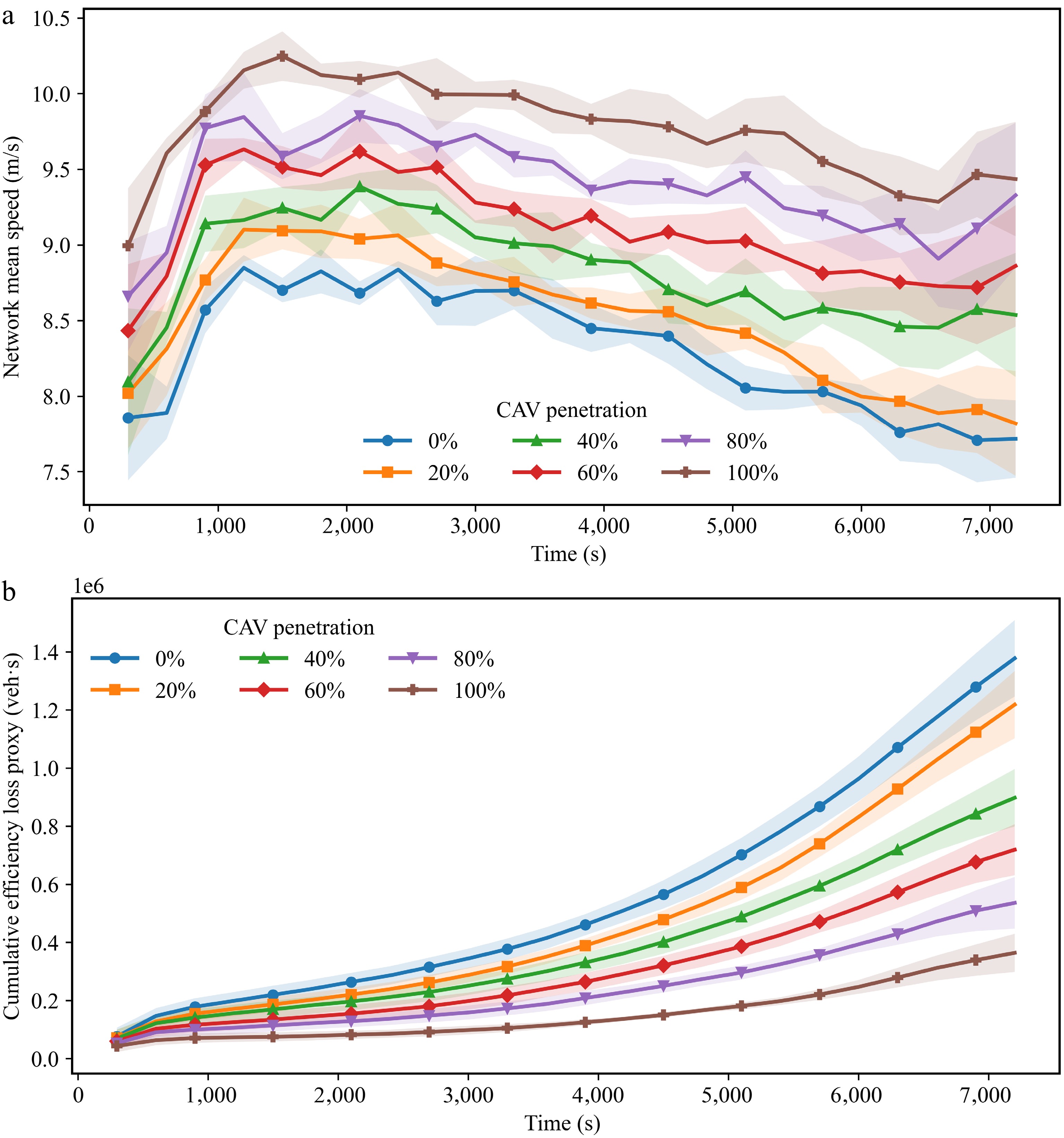
Figure 7. 

Temporal speed degradation and cumulative efficiency loss under different CAV penetration rates. (a) Network mean speed. (b) Cumulative efficiency loss.

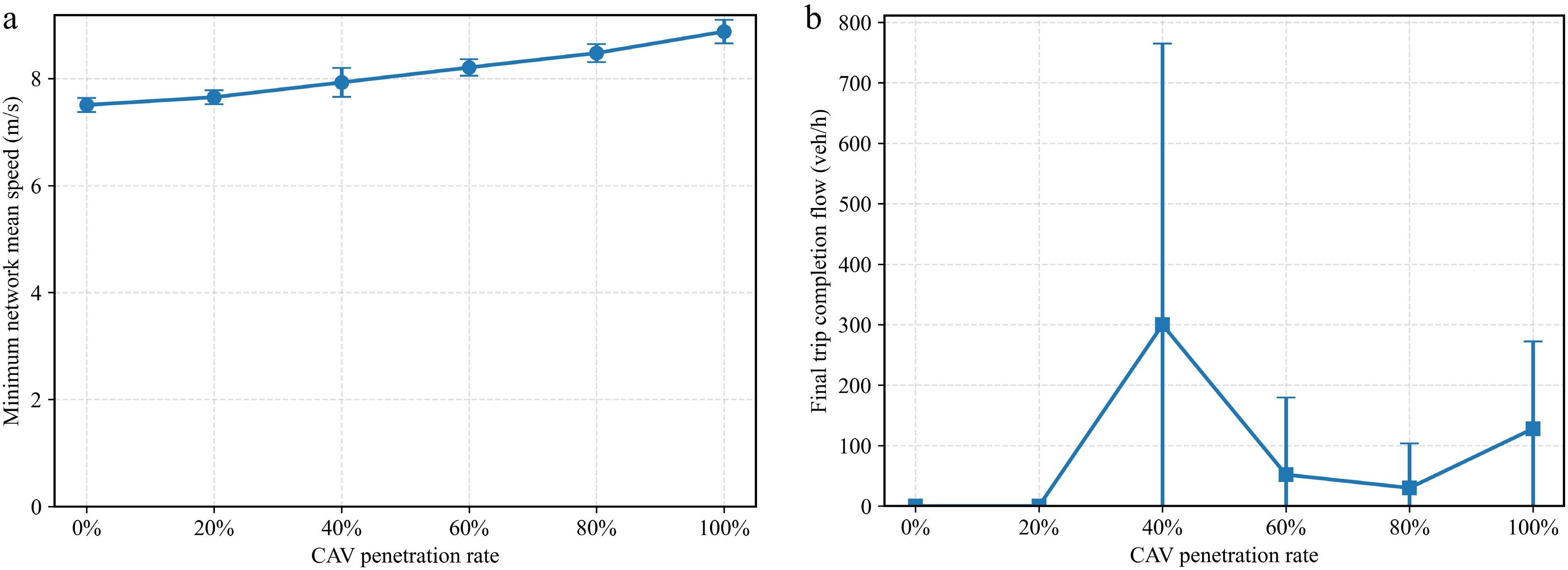
Figure 8. 

Robustness and terminal performance across penetration scenarios. (a) Minimum network mean speed. (b) Final trip completion flow.

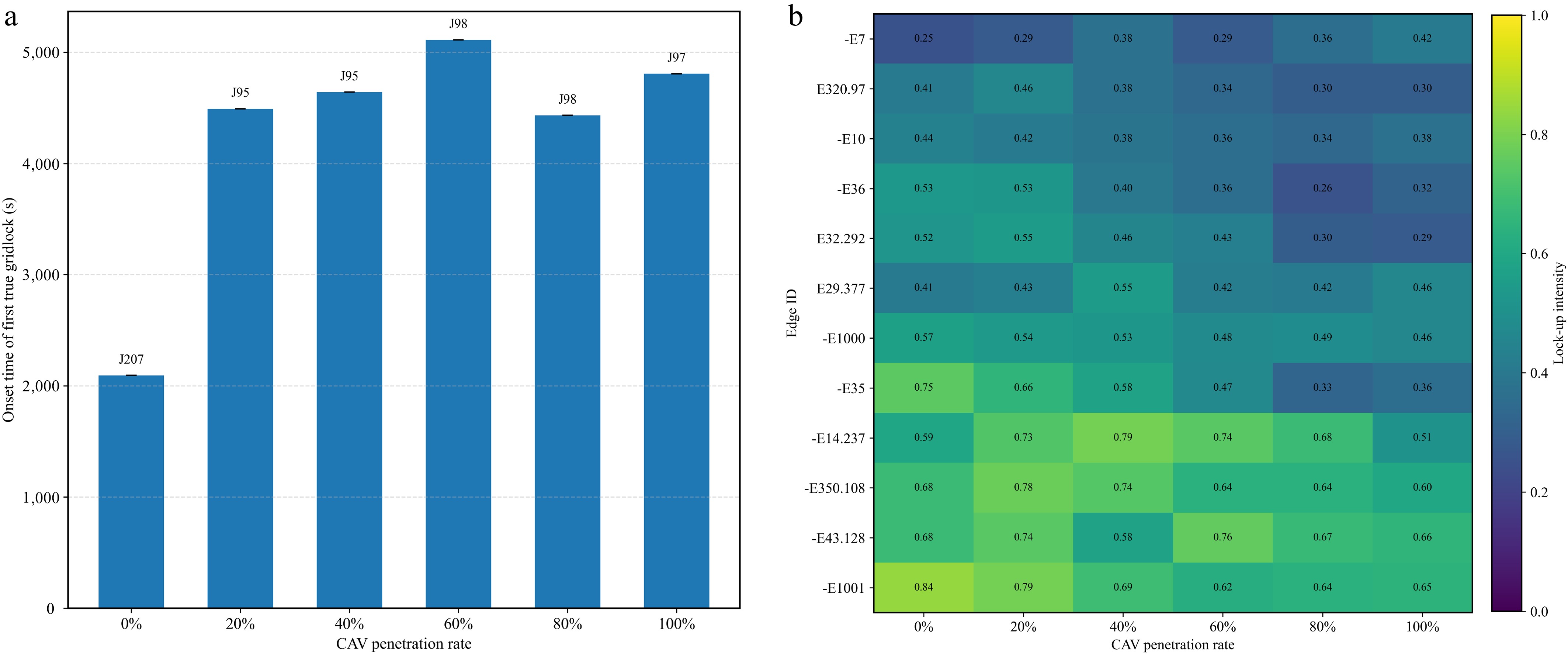
Figure 9. 

Spatial distribution of bottleneck probability and lock-up intensity in Network 1. (a) First detected gridlock onset time across penetration scenarios. (b) Lock-up intensity across penetration scenarios.

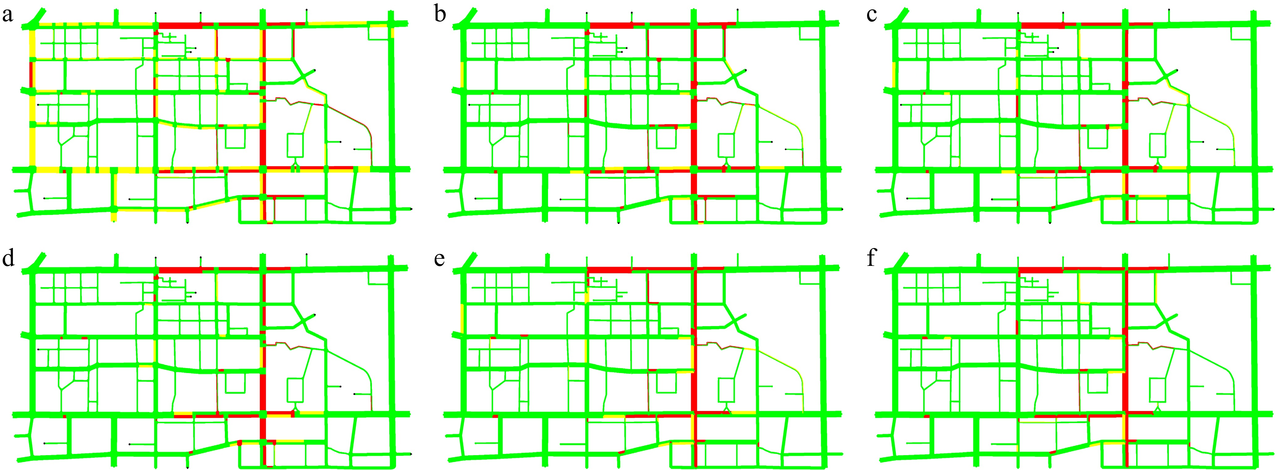
Figure 10. 

Representative spatiotemporal propagation of gridlock in Network 1. (a) Gridlock propagation at 0% CAV penetration. (b) Gridlock propagation at 20% CAV penetration. (c) Gridlock propagation at 40% CAV penetration. (d) Gridlock propagation at 60% CAV penetration. (e) Gridlock propagation at 80% CAV penetration. (f) Gridlock propagation at 100% CAV penetration.

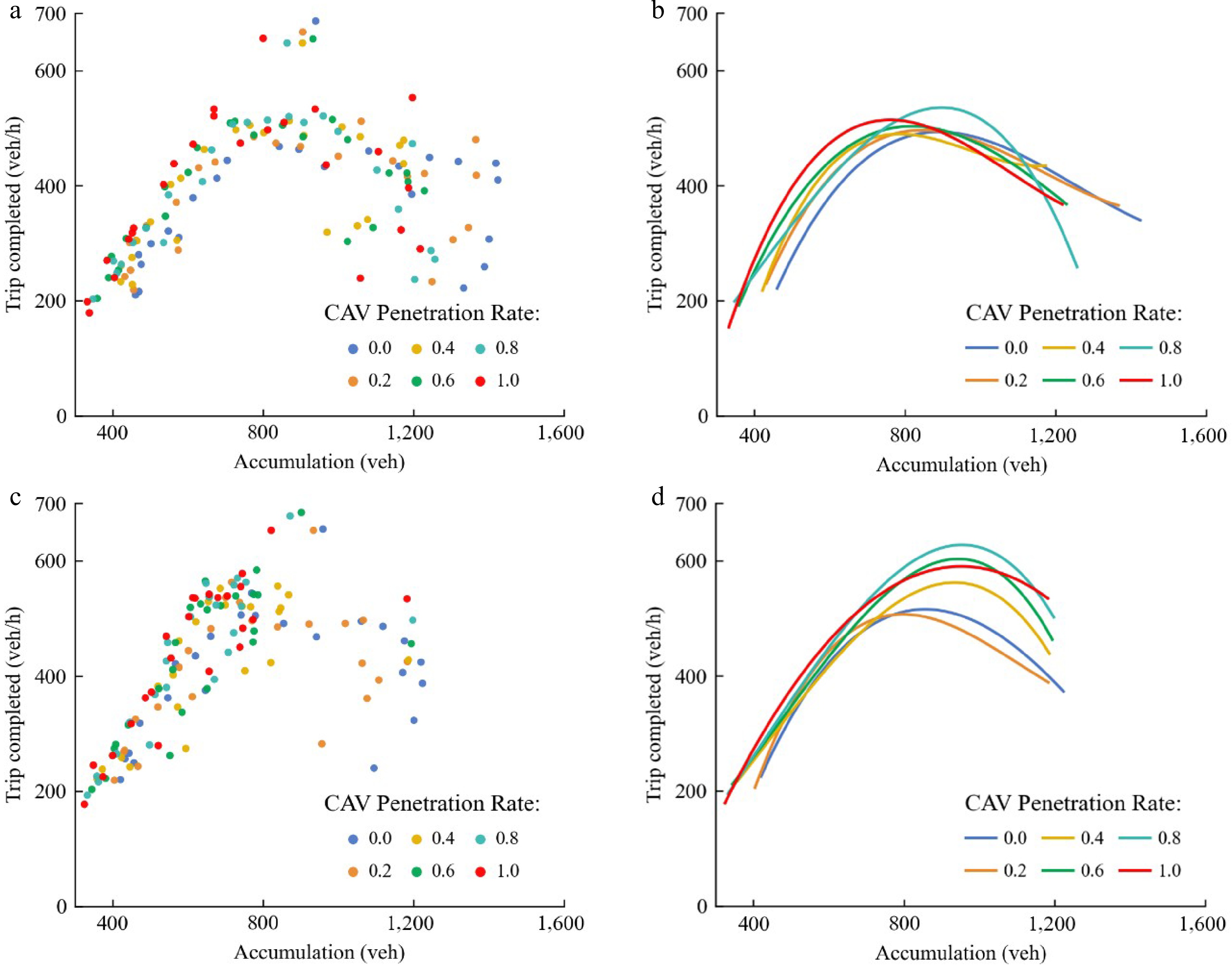
Figure 11. 

MFD trajectories and fitted curves of Network 1 and Network 2 under the same loading framework. (a) MFD trajectories in Network 1. (b) Fitted curve in Network 1. (c) MFD trajectories in Network 2. (d) Fitted curve in Network 2.