Analysis of gridlock risks in mixed traffic flow on heterogeneous urban road networks under oversaturation conditions

As global urbanization continues to accelerate, the increasing concentration of population and economic activities in cities has placed growing pressure on urban road traffic systems^[1,2]. The contradiction between limited road supply and steadily growing travel demand has intensified, making traffic congestion a 'chronic disease' of modern cities^[1]. Particularly during morning and evening commute peaks, urban road networks remain in saturated or even oversaturated conditions for extended periods, where local disturbances can easily trigger large-scale traffic jams, severely affecting urban efficiency and residents' travel quality^[3,4]. In this context, a deeper understanding of the propagation mechanism of traffic congestion in saturated urban networks is of great theoretical value and practical significance for developing effective traffic control strategies and improving network resilience^[5].

Meanwhile, urban traffic systems are undergoing a gradual transition from homogeneous traffic dominated by human-driven vehicles (HDVs) to heterogeneous mixed traffic in which HDVs and connected and autonomous vehicles (CAVs) coexist. In this study, heterogeneity is considered from three interrelated perspectives: network-structure heterogeneity, arising from the coexistence of arterials, sub-arterials, local streets, and residential branch roads with different operational roles; traffic-composition heterogeneity, resulting from the coexistence of HDVs and CAVs with different behavioral mechanisms; and spatiotemporal heterogeneity in congestion evolution, reflected in the uneven distribution of lock-up and congestion across the network. Traditionally, congestion in urban networks has been closely associated with intersection bottlenecks and local interaction mechanisms. For example, Qi et al. analyzed the formation and probability of intersection traffic deadlock^[6], while Huang modeled gridlock at roundabouts and showed how local lock-up conditions may emerge under constrained traffic operations^[7]. With the introduction of CAVs, the heterogeneity of traffic flow has become more prominent. Fakhrmoosavi et al. investigated the impacts of CAVs distributed over large-scale networks^[8], and Qin et al. developed an LWR model for mixed traffic flow in connected and autonomous vehicular environments^[9]. These studies indicate that traffic composition can substantially influence both local vehicle interactions and network-level traffic states.

At the macroscopic level, researchers have increasingly used the macroscopic fundamental diagram (MFD) to describe the aggregate state of urban road networks. Geroliminis & Daganzo^[10] provided empirical evidence for the existence of urban-scale MFDs, laying the foundation for macroscopic network analysis. Xu & Gayah further showed that hierarchical streets may make the free-flow branch of the MFD non-unimodal and non-concave^[11], while Buisson & Ladier found that separating central signalized streets from residential streets is important for obtaining a low-scatter MFD^[12]. In parallel, studies on mixed traffic have shown that increasing CAV penetration may affect urban network capacity, critical accumulation, and hysteresis characteristics of traffic states. Lu et al. showed that autonomous vehicles can improve urban network capacity^[13], Huang et al. characterized their impacts on MFDs^[14], and Lu et al. analyzed the hysteresis characteristics of MFD-based mixed traffic flow on expressways^[15].

Despite these advances, several gaps remain. First, many existing studies still rely on simplified arterial-based network representations or implicitly assume network homogeneity, which may underestimate the effects of local and residential streets on effective capacity and gridlock risk^[11,12]. Second, although the impacts of CAVs on traffic performance have been widely discussed, less attention has been paid to how mixed traffic affects gridlock-related risks in heterogeneous urban networks under strongly oversaturated demand^[13,14]. Third, the combined influence of network heterogeneity and traffic-composition heterogeneity has not yet been sufficiently incorporated into a unified analytical framework for gridlock-risk assessment.

To address these problems, this study investigates gridlock risks in mixed traffic flow on heterogeneous urban road networks under saturated and oversaturated conditions. A macro–micro coupled analytical framework is developed, in which the MFD is used to characterize network-level state evolution, while microscopic simulation is adopted to capture the behavioral differences between HDVs and CAVs and their operational implications. In addition, two network representations, namely a full network including local and residential streets and a simplified arterial-based benchmark network, are compared to examine how network representation affects macroscopic performance characterization and gridlock-risk assessment.

The contributions of this study are summarized as follows:

(1) A macro–micro coupled analytical framework is developed for investigating gridlock risks in oversaturated mixed traffic flow on heterogeneous urban road networks.

(2) The effects of different CAV penetration rates on gridlock occurrence, temporal deterioration, and spatial concentration are systematically examined under strongly unstable oversaturated conditions.

(3) A signal-cycle-based gridlock identification criterion and a probability-based bottleneck localization method are proposed to determine when and where gridlock is most likely to emerge and persist in heterogeneous networks. The rest of the paper is organized as follows. Literature review summarizes the relevant literature. Methodology presents the proposed methodological framework, including the microscopic mixed-traffic simulation, the MFD-based macroscopic description, and the gridlock analytics module. Case study introduces the case study and empirical results. Finally, Conclusions concludes the paper.

Gridlock represents one of the most severe forms of operational failure in urban traffic systems under saturated or oversaturated demand. Unlike ordinary congestion at isolated intersections, gridlock involves a broader loss of effective network discharge, characterized by persistent queues across signal cycles, rapid vehicle accumulation, and substantially reduced outflow.

Several studies have examined this problem from the perspective of local lock-up and network-wide failure. Qi et al. modeled intersection traffic deadlock formation and estimated its probability through a Petri net-based approach, showing that local conflicts may trigger persistent blockage under certain traffic conditions^[6]. Huang focused on roundabouts and modeled gridlock formation at this special facility type, demonstrating that severe lock-up can also emerge from local interaction mechanisms rather than only from corridor-level oversaturation^[7]. At the network scale, Mahmassani et al. systematically discussed the theory, characteristics, and dynamics of urban network gridlock and emphasized that gridlock should be understood as a sustained failure of network operations rather than a temporary traffic disturbance^[16]. Mendes et al. also investigated traffic gridlock on complex networks and highlighted that network structure itself can influence the emergence of lock-up states^[17]. Daganzo described urban gridlock through a macroscopic modeling framework and showed that lock-up can be understood and mitigated at the neighborhood or city scale^[18].

In addition, some studies have interpreted congestion evolution from the perspective of network spreading. Saberi et al. found that the spreading of traffic jams in urban networks can be described by a simple contagion process^[19], while Ashfaq further discussed traffic congestion as a spreading phenomenon. Although these studies mainly focus on congestion spreading rather than gridlock risk itself^[20], they indicate that severe congestion in urban networks cannot be understood only at the level of individual links or intersections.

Overall, existing studies provide an important basis for understanding severe congestion and network lock-up. However, many of them focus either on local deadlock behavior or on abstract network dynamics. Relatively few studies have assessed gridlock risk in heterogeneous urban road networks that simultaneously involve arterial roads, local streets, and mixed traffic conditions.

MFD-based studies and network representation

At the macroscopic level, the MFD has become a widely used tool for describing the aggregate operating state of urban road networks. Geroliminis & Daganzo provided the seminal empirical evidence for the existence of urban-scale MFDs, showing that network accumulation and network performance can exhibit a stable aggregate relationship^[10]. This work established the MFD as an important framework for traffic-state monitoring and large-scale control.

Subsequent studies showed that the quality of an MFD depends strongly on network homogeneity. Geroliminis & Sun investigated the properties of a well-defined MFD and pointed out that low-scatter MFDs should not be universally expected for all urban networks^[21]. Xu & Gayah demonstrated that hierarchical streets may cause the free-flow branch of the MFD to become non-unimodal and non-concave when route choice follows a user-equilibrium principle^[11]. Buisson & Ladier further found that network heterogeneity has a strong influence on the MFD shape, and that separating central signalized streets from more residential streets is an important condition for obtaining a low-scatter MFD^[12]. Ramezani et al. further examined the dynamics of heterogeneity in urban networks and showed that heterogeneity plays an important role in MFD scatter, hysteresis, and hierarchical traffic control^[22]. Ambühl et al. combined percolation theory with the MFD and suggested that network-level congestion states are closely related to structural vulnerability and spatial heterogeneity^[23].

These studies suggest that MFD-based analysis depends not only on how macroscopic traffic states are described, but also on how the network itself is represented. In many existing studies, the network is simplified by keeping only arterial and sub-arterial roads, while local and residential streets are excluded. Although such simplification may be acceptable in some control-oriented applications, it may underestimate vehicle storage effects, local spillback interactions, and effective-capacity constraints associated with fine-grained branch-road structures. Therefore, network representation is directly related to the interpretation of MFDs and to the assessment of gridlock risk under oversaturated conditions.

Mixed traffic flow and the impacts of CAVs

The increasing deployment of CAVs has made mixed traffic flow a central issue in traffic-flow research. Compared with conventional homogeneous traffic, mixed traffic involves substantial differences in reaction time, control precision, car-following behavior, and lane-changing logic across vehicle types, which may reshape both local vehicle interactions and aggregate system performance.

Several studies have examined these effects from modeling and simulation perspectives. Fakhrmoosavi et al. investigated the impacts of connected and autonomous vehicles over large-scale networks and showed that spatially distributed heterogeneous drivers can significantly affect network traffic states^[8]. Qin et al. proposed an LWR model for mixed traffic flow in connected and autonomous vehicular environments, providing a macroscopic description of heterogeneous traffic composition^[9]. Talebpour & Mahmassani analyzed the influence of connected and autonomous vehicles on traffic-flow stability and throughput, showing that higher CAV penetration can improve string stability and increase throughput^[24]. Stern et al. further provided field-experimental evidence that even a very small number of autonomous vehicles can dampen stop-and-go waves, suggesting that low penetration rates may still alter traffic stability^[25]. Mohajerpoor & Ramezani analytically examined mixed streams and showed that traffic composition and vehicle arrangement may substantially affect headway distribution and capacity-related characteristics^[26].

At the operational level, Lu et al. used a microscopic traffic simulation to show that increasing the penetration rate of autonomous vehicles can improve urban network capacity^[13]. Huang et al. examined the impacts of autonomous vehicles on MFDs and found that CAVs may increase capacity but also influence the critical accumulation of the system^[14]. Lu et al. analyzed MFD-based mixed traffic flow on expressways and showed that increasing CAV penetration can weaken hysteresis effects, although the improvement may not be strictly linear at high penetration levels^[15].

At the microscopic modeling level, Treiber et al. discussed congested traffic states in microscopic simulations and provided a classical basis for vehicle-level traffic modeling^[27]. Xiao et al. proposed realistic car-following models for adaptive cruise control and cooperative adaptive cruise control vehicles, making it possible to simulate CAV behavior more realistically in mixed traffic^[28]. Silgu et al. further investigated mixed traffic involving cooperative adaptive cruise-controlled and human-driven vehicles in SUMO, showing that different control assumptions may substantially affect traffic performance^[29].

Taken together, these studies suggest that CAV penetration may influence traffic stability, capacity, and macroscopic traffic states. However, most existing work focuses on general performance indicators such as throughput, delay, or hysteresis. However, less attention has been paid to how different CAV penetration rates affect gridlock-related risks in oversaturated urban road networks, particularly when network structure is itself heterogeneous.

Research gaps and motivation of this study

Overall, existing studies provide a solid foundation for understanding severe congestion, MFD-based network analysis, and the operational impacts of mixed traffic flow. However, several limitations remain. First, many MFD-based studies still rely on simplified network representations or assume relatively homogeneous traffic environments, which may underestimate the role of local and residential streets in vehicle storage, effective capacity reduction, and severe lock-up conditions^[11,12]. Second, although previous studies have examined gridlock either from local operational perspectives or from aggregate network viewpoints, relatively few studies connect these two levels in a unified framework for heterogeneous urban networks under oversaturated demand^[6,7,16,17]. Third, while many studies have explored the benefits of CAVs in terms of stability, capacity, and MFD characteristics^{[13−15,24−26]}, the combined impacts of network heterogeneity and traffic-composition heterogeneity on gridlock risks have not yet been systematically clarified.

Motivated by these limitations, this study focuses on mixed traffic flow in heterogeneous urban road networks under saturated and oversaturated conditions. The objective is to evaluate how network representation and CAV penetration jointly affect gridlock occurrence, temporal deterioration, and the spatial concentration of severe lock-up conditions. To this end, a macro–micro coupled analytical framework is adopted, in which the MFD is used to characterize network-level state evolution, while microscopic simulation is used to capture the behavioral differences between HDVs and CAVs and their implications for operational risks.

To analyze gridlock risks in oversaturated mixed traffic flow on heterogeneous urban road networks, this study proposes a hierarchical analytical framework under different network representations. As shown in Fig. 1, this framework mainly consists of the following steps:

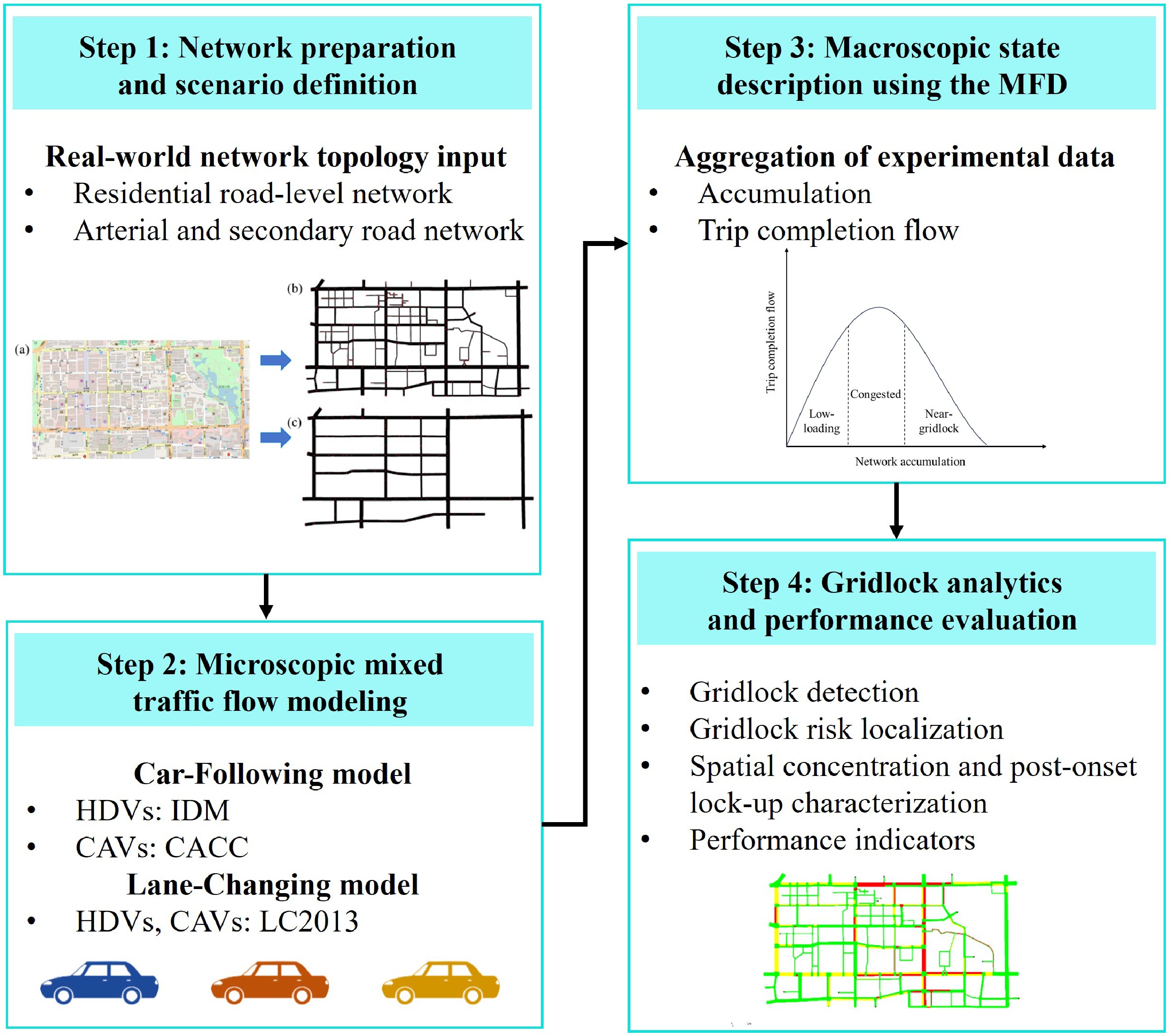
Figure 1. 

Overall analytical framework.

● Network preparation and scenario definition: Following previous simulation-based studies of CAV impacts on urban traffic networks^[13], two network representations are developed to capture different levels of topological granularity: (1) a full network that includes local and residential streets, and (2) a simplified network focused on arterial roads. Signal control parameters and travel demand configurations are calibrated to ensure consistency and comparability across all scenarios.

● Microscopic mixed-traffic simulation modeling: Mixed traffic flow is simulated by integrating a car-following model that differentiates HDVs and CAVs and a lane-changing model that captures discretionary and mandatory maneuvers. Behavioral parameters are set according to vehicle type and scenario assumptions, so that both local interactions and lane-level dynamics are represented.

● Macroscopic state description using the MFD: Network-level traffic states are aggregated over the whole network to obtain macroscopic variables such as network accumulation, trip completion flow, and mean speed. Based on these variables, an MFD-based representation is adopted to describe the evolution of network performance and to support cross-scenario comparisons at the macroscopic level.

● Gridlock analytics and performance evaluation: Based on microscopic trajectories and aggregated network states, gridlock occurrence is detected, the onset time and high-risk bottlenecks are identified, and the post-onset spatial concentration of lock-up conditions is characterized. Meanwhile, performance indicators, including network accumulation, trip completion flow, network mean speed, and cumulative efficiency loss, are used to quantify the severity of temporal deterioration under different network representations and CAV penetration scenarios.

Network preparation and scenario definition

To examine how network representation affects macroscopic state characterization and gridlock risks, we construct two network representations that reflect different levels of topological detail: a full network that explicitly includes residential street-level structures, and a simplified benchmark network that retains only arterial and sub-arterial roads, consistent with the minimal structures commonly adopted in MFD aggregation studies^[14].

Scenario inputs are defined using a controlled-comparison design to ensure the comparability of experimental outcomes across network representations. Specifically, signal control settings, demand settings, and routing rules are specified consistently across the two representations, while only the factors of interest (e.g., traffic composition, such as the penetration rate of CAVs) are varied. This design ensures consistent input configurations across scenarios, thereby allowing any observed differences in macroscopic performance or gridlock risk to be attributed solely to the network representation and traffic composition.

Unlike MFD-based studies that focus on stable or quasi-stable states, our scenario definition concentrates on system behaviors in a strongly unstable regime, in which demand is close to or exceeds the effective network discharge capacity and congestion may rapidly transition into severe spillback and gridlock. Under such oversaturated conditions, the system provides sufficient stress to reveal structural vulnerabilities and to support the subsequent analysis of gridlock onset, spatial concentration, and propagation.

Microscopic mixed-traffic simulation modeling

To explicitly summarize the construction of the microscopic simulation, we represent the microscopic Simulation Analysis Module (SAM) as a composition of the car-following model, the lane-changing model, and basic traffic rules (e.g., signal compliance, right-of-way/yielding, and collision avoidance constraints):

where, $ {\mathcal{F}}_{\text{CF}}\left(\cdot \right) $ and $ {\mathcal{F}}_{\text{LC}}\left(\cdot \right) $ denote the car-following and lane-changing mechanisms parameterized by $ {\mathbf{\Theta }}_{\text{CF}} $ and $ {\mathbf{\Theta }}_{\text{LC}} $, respectively, and $ \mathcal{R} $ denotes a set of simple traffic rules enforced in the simulator (e.g., obeying traffic signals, yielding/priority rules at conflicts, and safety constraints). This formulation clarifies that network-level trajectories and performance measures are generated by the joint effects of longitudinal interactions, lateral maneuvers, and rule-based constraints.

Car-following model

The IDM model proposed by Treiber et al. is used to describe the car-following behavior of HDVs^[27]:

where, a is the acceleration of the subject vehicle; a_max is the maximum acceleration; $ v $ is the current speed of the subject vehicle; $ {v}_{0} $ is the desired speed, generally the speed limit of each road segment; $ {s}^{*}\left(v,\Delta v\right) $ is the desired safe distance; s is the actual gap; s₀ is the standstill distance between the subject vehicle and its leader under saturation conditions; s₁ is the speed-dependent spacing under congested conditions; T is the desired time headway; $ \Delta v $ is the speed difference between the subject vehicle and its leader; and b is the desired deceleration.

In this study, CAVs are controlled using the cooperative adaptive cruise control (CACC) model. The car-following model proposed by Xiao et al. is adopted^[28]:

where, n is a vehicle, e_n is the difference between the actual spacing and the desired spacing; $ \dot{{e}_{i}} $ is the temporal derivative of spacing difference. $ {v}_{n} $ is the speed of the following vehicle; $ {v}_{n,next} $ is the vehicle speed at the next time step; t_d is the desired time headway; control gain k₁ is the weight on spacing error; and control gain k₂ is the weight on the derivative of spacing error.

It should be noted that the present study parameterizes microscopic behavior at the vehicle-class level rather than defining separate interaction-specific models for all possible leader–follower pairings (e.g., HDV→HDV, HDV→CAV, CAV→HDV, and CAV→CAV). Under this implementation, however, all four pairings still arise naturally during simulation because HDVs and CAVs coexist in the same traffic stream. When a following relationship is formed, the following vehicle applies the car-following logic associated with its own vehicle class, while the leader's state enters the interaction dynamically through spacing, speed, and relative speed. Therefore, mixed pairings are not excluded; they are generated endogenously in the simulated traffic stream. This vehicle-class-based implementation is adopted to preserve parsimony and comparability across scenarios, because the objective of this study is to examine network-level gridlock risk under oversaturated mixed traffic conditions rather than to exhaustively represent all interaction-specific behavioral regimes. We acknowledge that this simplification may influence some fine-scale microscopic interaction details, but it is unlikely to change the central comparative findings drawn from repeated-run network-level analysis.

Lane-changing model

Both CAVs and HDVs adopt the LC2013 model. In this study, we use two willingness parameters to explicitly represent behavioral differences in mixed traffic flow: L_s for self-initiated lane changes and L_c for cooperative lane changes. A lane change can be executed only when a feasible opportunity exists (i.e., safety constraints such as a sufficient gap are satisfied). Given feasibility, we describe the triggering logic in a simple and interpretable form.

For discretionary lane changes, the vehicle is more likely to change lanes when the target lane offers a speed advantage. We define a benefit measure:

where, $ {v}_{\text{cur}} $ is the vehicle's expected speed if it stays in the current lane and $ {v}_{\text{tar}} $ is the expected speed on the target lane. A discretionary lane change is triggered when:

where, θ_d is a threshold. Thus, a larger L_s means the vehicle is more willing to initiate discretionary lane changes under the same potential speed gain.

For cooperative lane changes, the lane change may require surrounding vehicles (typically the target-lane follower) to yield. We quantify the required cooperation by:

where, $ {v}_{\text{fol}} $ is the current speed of the target-lane follower and $ v_{\text{fol}}^{\text{safe}} $ is the maximum speed at which the follower can maintain a safe gap if the subject vehicle merges. Cooperation is considered sufficient when:

where, θ_c is a threshold. A larger L_c indicates stronger cooperation willingness, meaning that surrounding vehicles are more likely to yield (within safety limits), which facilitates lane changes.

Macroscopic state description using the MFD

The MFD is used in this study as an aggregated representation of network-level traffic states. Rather than adopting the conventional density–flow form, we describe the MFD by the relationship between network accumulation and trip completion flow, because this form is more directly related to the buildup of congestion, the degradation of discharge performance, and the onset of gridlock under oversaturated conditions.

Let n(t) denote the number of vehicles present in the network at time t, i.e., the network accumulation, and let G(t) denote the trip completion flow, i.e., the number of completed trips per unit time. The MFD is then expressed in the following aggregated form:

where, Φ(·) represents the macroscopic discharge characteristics of the network. In practice, the observed state pairs (n(t),G(t)) over time constitute the empirical MFD trajectory.

Figure 2 provides a schematic illustration of the MFD in the accumulation–completion-flow plane. In general, when accumulation is low, trip completion flow increases as more vehicles enter the network and the utilization of available road space improves. As accumulation continues to grow, the network gradually approaches its effective operating limit. Beyond this range, further accumulation is no longer associated with better throughput; instead, trip completion flow tends to stabilize and then decline as queues expand, spillback interactions strengthen, and discharge efficiency deteriorates. Under strongly oversaturated conditions, the network may eventually enter a low-discharge state characterized by high accumulation and weak output, which is closely associated with severe congestion and near-gridlock conditions.

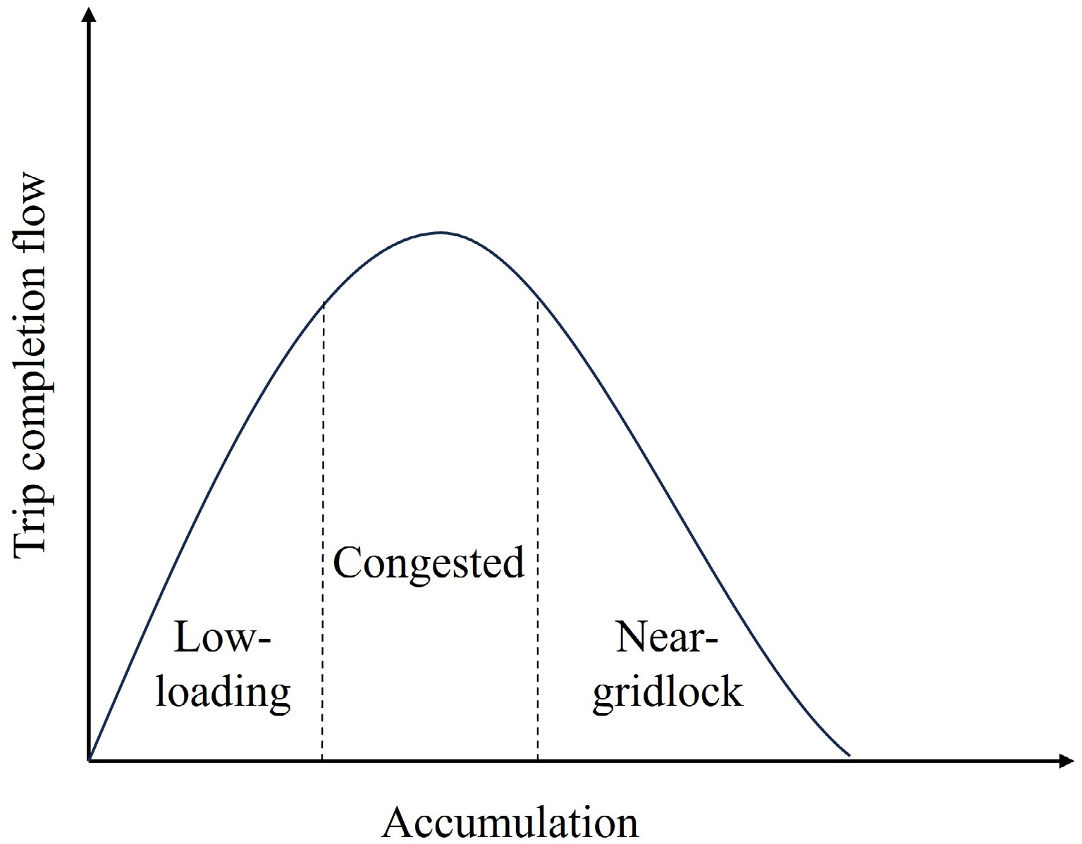
Figure 2. 

Macroscopic fundamental diagram.

Compared with density-based formulations, the accumulation–completion-flow representation is more suitable for the objectives of this study. First, it directly reflects whether the network can still convert stored vehicles into completed trips under oversaturated demand. Second, it is naturally connected to the subsequent analyses of temporal deterioration, completion-flow reduction, and terminal performance. Therefore, the MFD is used here not as a strict deterministic law, but as a compact macroscopic description of how network storage and discharge interact during congestion evolution.

To reduce the influence of short-term fluctuations, the state variables are aggregated over fixed time intervals. Let n_τ denote the network accumulation in interval τ, and let G_τ denote the corresponding trip completion flow. The empirical MFD is then obtained from the sequence of observed state pairs (n_τ,G_τ). For descriptive purposes, the overall relationship may be approximated by a fitted curve:

where, θ is the parameter vector to be estimated. In this study, the fitted curve is used only to summarize the overall macroscopic envelope, while the scatter of state points is interpreted as an important manifestation of stochasticity and heterogeneity in oversaturated mixed traffic flow. In this study, the fitted curve is used only to summarize the overall empirical envelope of the observed MFD trajectory, rather than to represent a strict theoretical law. This treatment is consistent with the MFD literature, in which no universally accepted functional form has been established, and different formulations may be adopted for different analytical purposes; see, for example, Ambühl et al., who proposed a functional form with physical meaning for the MFD. Therefore, the fitted curve is interpreted here only as an auxiliary descriptive tool^[30].

Gridlock analytics and performance evaluation

To connect the microscopic simulation results with the macroscopic state evolution described by the MFD, this study develops a gridlock analytics and performance evaluation module. The purpose of this module is not only to determine whether gridlock occurs, but also to identify when and where it first emerges, how it propagates through the network, and how severely it degrades network performance over time. Accordingly, the analysis combines intersection-level gridlock detection, bottleneck localization, propagation tracking, and system-level performance measurement within a unified framework.

More specifically, the proposed procedure includes four components. First, gridlock onset is identified at candidate bottleneck intersections using a signal-cycle-based criterion that captures persistent low-speed, high-saturation, and low-discharge states. Second, repeated simulations are used to estimate the empirical occurrence probability of gridlock at each monitored location, so that structurally vulnerable bottlenecks can be distinguished from purely random realizations. Third, after the first onset of gridlock, the spatiotemporal propagation of congestion is characterized by tracking the persistence and concentration of lock-up conditions on critical links and intersections. Finally, a set of macroscopic and travel-efficiency indicators, including network mean speed, accumulation growth, trip completion flow, and cumulative efficiency loss, is used to quantify the severity and robustness of network operations under different scenarios.

Step 1: Gridlock detection

To improve the robustness of gridlock identification, this study does not rely solely on local vehicle immobility. Instead, gridlock is defined as a persistent intersection-level state characterized by simultaneous low speed, high occupancy, and low discharge over at least one full signal cycle. This formulation is intended to distinguish true spillback-induced lock-up from temporary stops caused by signal control or short-term queueing.

Let $ \mathcal{I} $ denote the set of monitored intersections (candidate bottlenecks). For each intersection $ i\in \mathcal{I} $, let $ {\mathcal{L}}_{i} $ denote the set of its incoming links. At time t, three weighted intersection-level indicators are defined as follows:

where, $ {v}_{l}\left(t\right) $ is the mean speed on incoming link l, k_l(t) is the density on link l, q_l(t) is the discharge flow on link l, $ k_{l}^{\text{jam}} $ is the jam density of link l, and $ q_{l}^{\text{cap}} $ is the reference discharge capacity of link l. The weight w_l reflects the relative importance of each incoming link and can be specified by link length, lane number, or their combination.

Based on these indicators, the gridlock state of intersection i is defined by the following indicator function:

where, $ {v}_{\text{th}} $ is the low-speed threshold, o_th is the high-occupancy (or high-density) threshold, q_th is the low-discharge threshold, and C_i is the signal cycle length at intersection i. Thus, gridlock is declared only when the intersection remains in a low-speed, high-saturation, and low-discharge state continuously over one complete signal cycle.

Accordingly, the onset time of gridlock at intersection i is given by:

and the onset time of the first gridlock event in one simulation run is:

This criterion captures the essential operational characteristic of gridlock, namely, that vehicles remain highly accumulated near the intersection while the effective discharge capacity cannot recover within a full signal cycle. Compared with a pure immobility-based criterion, it is less sensitive to short red-light stops and therefore provides a more reliable basis for onset-time detection, bottleneck localization, and subsequent propagation analysis. Therefore, the proposed criterion should be interpreted as an operational definition of persistent local lock-up, which serves as the basis for subsequent network-level gridlock analysis rather than as a direct claim of instantaneous whole-network collapse.

Step 2: Gridlock risk localization

Since gridlock under oversaturated mixed traffic flow is influenced by stochastic factors such as route realization, vehicle interactions, and heterogeneous CAV–HDV composition, a single simulation run is not sufficient to identify structurally vulnerable bottlenecks. Therefore, each scenario is repeated over multiple runs with different random seeds, and the empirical occurrence frequency of intersection-level gridlock is used to localize high-risk bottlenecks.

Let $ R $ denote the total number of repeated runs for a given scenario, and let $ t_{i,r}^{g} $ denote the detected onset time of gridlock at intersection i in run r. Define the indicator:

which equals 1 if gridlock is detected at intersection i in run r, and 0 otherwise. The empirical gridlock probability of intersection i is then defined as:

A larger value of $ P_{i}^{g} $ indicates that the corresponding intersection is more likely to act as a recurrent bottleneck under the given scenario. In this study, intersections with relatively high $ P_{i}^{g} $ are identified as high-risk bottlenecks. This probability-based localization emphasizes structural vulnerability and repeated instability, rather than relying on a single realization of congestion. In addition, for those intersections that experience gridlock in multiple runs, the distribution of $ t_{i,r}^{g} $ can be further used to summarize the typical onset timing of bottleneck activation.

Step 3: Spatial concentration and post-onset lock-up characterization

After the first onset of gridlock is identified, the next task is not to reconstruct the full time-resolved spreading frontier, but to characterize the post-onset spatial concentration and persistence of lock-up conditions in the network. This step is intended to identify which links and intersections remain most severely affected after gridlock emerges and to infer the dominant bottleneck corridors associated with congestion propagation.

Let t^g denote the onset time of the first gridlock event in one simulation run. For each link l, define a lock-up indicator:

where, $ {v}_{l}\left(t\right) $ is the link mean speed at time t, k_l(t) is the link density, $ k_{l}^{\text{jam}} $ is the jam density, $ v_{l}^{\text{th}} $ is the low-speed threshold, and $ o_{l}^{\text{th}} $ is the normalized occupancy (or density) threshold. Thus, $ {z}_{l}\left(t\right)=1 $ indicates that link l is in a lock-up-like state at time t.

To measure how persistently a link remains affected after the onset of gridlock, the lock-up intensity of link l is defined as:

where, T is the total simulation time. In discrete form:

where, τ_g is the first interval after gridlock onset and N_g = N − τ_g + 1. A larger I_l indicates that link l remains in a lock-up state for a larger fraction of the post-onset period.

Based on the spatial distribution of $ {I}_{l} $ and the corresponding bottleneck intersections, this study identifies the dominant corridors and local concentrations of post-gridlock lock-up. Therefore, Step 3 does not aim to recover the exact time-varying spreading frontier, but rather to provide a robust spatial characterization of where severe lock-up persists after gridlock has emerged.

Step 4: Performance indicators

To evaluate the severity of network deterioration under different CAV penetration scenarios, this study uses a set of macroscopic performance indicators that are consistent with the accumulation–trip-completion-flow representation. Specifically, network accumulation, trip completion flow, network mean speed, and cumulative efficiency loss are used to quantify the temporal degradation and residual performance of the system.

The network accumulation at time t, denoted by n(t), is defined as the total number of vehicles present in the network. The trip completion flow, denoted by G(t), is defined as the number of completed trips per unit time. These two variables jointly describe the macroscopic loading and discharge states of the network. In general, rapid growth in accumulation together with a decline in trip completion flow indicates that vehicles are being stored in the network faster than they can be discharged, implying an increasing risk of spillback and gridlock.

The network mean speed is computed as the weighted average of link mean speeds:

where, $ {v}_{l}\left(t\right) $ is the mean speed on link $ l $, $ \mathcal{L} $ is the set of network links, and w_l is the weight associated with link l. In this study, the network mean speed is used to characterize the overall operating condition of the network and to identify the extent of speed degradation during congestion development.

To quantify the cumulative impact of congestion over time, a proxy indicator of cumulative efficiency loss is defined as:

where, n_τ is the network accumulation in interval τ, $ {\bar{v}}_{\tau } $ is the network mean speed, $ {v}^{\text{ff}} $ is the reference free-flow speed, and Δt is the aggregation interval. A larger value of L(T) indicates more severe system-wide delay and lower overall operational efficiency.

These indicators are used in the subsequent analysis to examine temporal deterioration, including the evolution of accumulation and trip completion flow, the degradation of network mean speed, and the accumulation of efficiency loss under different penetration scenarios.

A simulation network was constructed based on the topology of a portion of Shenzhen's road network, as shown in Fig. 3. This study uses SUMO to construct the road network structures (Network 1 and Network 2) because it provides an open-source, microscopic traffic simulation environment with a complete toolchain for importing real-world road geometry, defining signal control and lane-level attributes, and generating demand. Moreover, SUMO outputs high-resolution vehicle trajectories and link/intersection performance measures, which are essential for identifying spillback and gridlock processes and for ensuring consistent, reproducible comparisons between different network representations under the same simulation settings. Network 1 contains 186 nodes and 524 links. Each link is one-way, and the network includes nearly all motor-vehicle roads shown in Fig. 3a. Such a structure implies that the overall network does not necessarily satisfy the characteristics of a homogeneous network. Network 2 contains 110 nodes and 248 links. It is derived from Network 1 by removing residential motor vehicle roads while retaining only arterial and sub-arterial roads. Meanwhile, the link segmentation is kept unchanged, i.e., the access and egress connections associated with the removed residential motor vehicle roads are preserved. Network 2 corresponds to the minimal network structure adopted by most MFD aggregation models. This design enables us to examine whether excluding lower-level roads changes the estimated gridlock probability, onset time, bottleneck concentration, and MFD characteristics under comparable loading conditions.

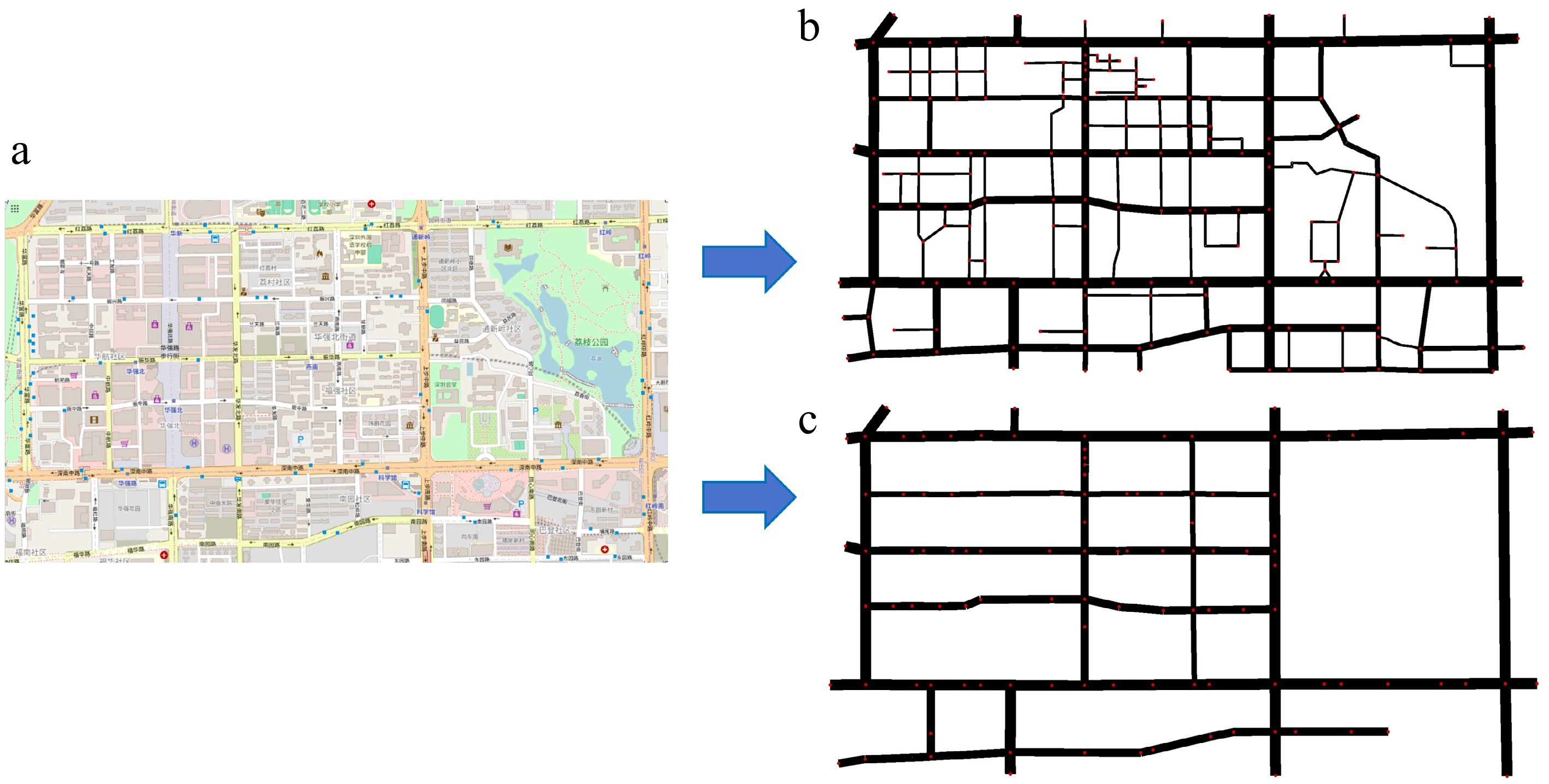
Figure 3. 

Simulation network. (a) The real-world network map, (b) Network 1, and (c) Network 2.

Demand loading and signal settings

Figure 4 shows the normalized stair-peak demand profile adopted in the simulations. The loading process consists of four consecutive stages: a low-demand stage, a stepwise rising stage, a sustained high-demand stage, and a falling stage. This profile is designed to gradually push the system from a relatively light-loading condition toward a strongly oversaturated regime, and then maintain high demand long enough to reveal congestion buildup, spillback interaction, and possible gridlock formation. Compared with a simple constant-demand setting, this staged loading profile is more suitable for observing the full temporal evolution of network deterioration and recovery. Therefore, this setting enables the observation of congestion and even gridlock phenomena. Both Network 1 and Network 2 adopted this demand-loading scheme.

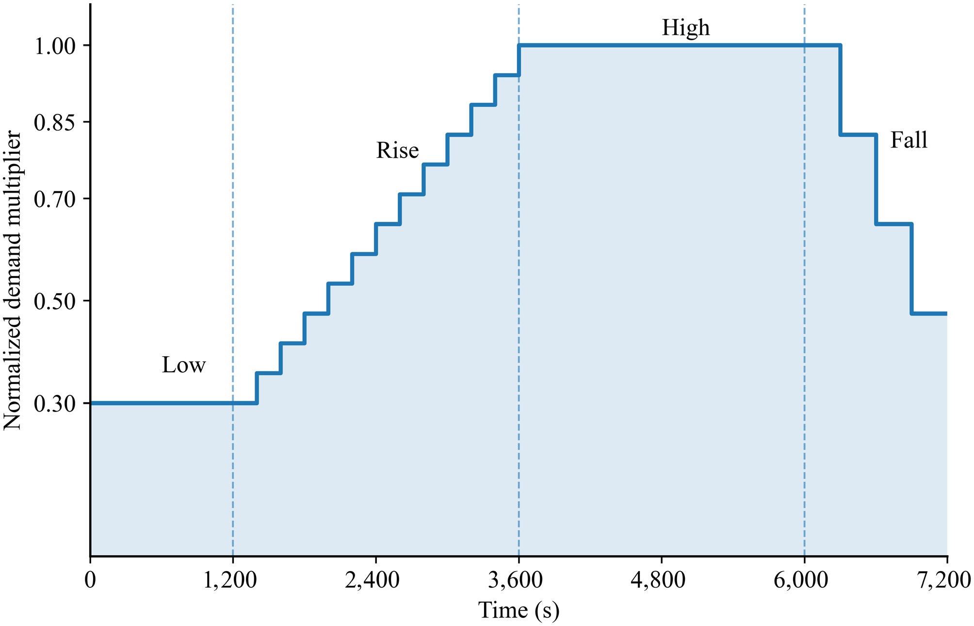
Figure 4. 

Demand-loading scheme.

All drivable roads with no upstream connections in the network are defined as source edges. Vehicles are only generated from source edges during the simulation to avoid introducing excessive traffic flow within the network. A Poisson process is adopted for vehicle generation, and the input flow is weighted and allocated according to the number of lanes of each source edge, ensuring that multi-lane roads carry higher input traffic volumes. The fundamental demand intensity at the network level is set based on the theoretical capacity of the road network: specifically, the total number of lanes of all source edges is summed, and the maximum allowable input flow of the network is calculated by combining the theoretical capacity of a single lane and the capacity utilization rate, as given by the following formula:

where, S is the set of all drivable source edges with no upstream motor vehicle connections in network n; m_e is the number of entrance lanes at source edge e; c₀ is the theoretical input capacity of a single lane; η is the capacity reduction factor, which accounts for the impacts of signal control, turning interference, and unbalanced lane utilization, etc.

To justify that the adopted demand profile places the system in a strongly unstable regime rather than in a clearly stable or fully collapsed state, we conducted a local demand sensitivity test around the baseline loading level D₀ in 0% penetration rates of CAVs. Demand sensitivity analysis of gridlock occurrence is shown in Table 1. The results showed that reducing the total demand by approximately 4% led to no gridlock in all repeated runs, whereas increasing the demand by approximately 4% resulted in inevitable gridlock. Therefore, the baseline loading level lies in the vicinity of the critical loading threshold, where small demand perturbations induce qualitatively different outcomes. This threshold-adjacent behavior indicates that the selected demand scheme places the network in a strongly unstable, oversaturated regime suitable for observing gridlock triggering, stochastic onset, and spatiotemporal propagation.

Because Network 2 is a simplified arterial-only representation derived from Network 1, directly imposing the same absolute demand on the two networks would confound representation effects with differences in effective input capacity. Therefore, source links were first defined separately for each network as motorized links without upstream incoming connections, and vehicles were inserted only from these source links. The insertion probability of each source link was weighted by its number of lanes. To make the two network representations comparable under equivalent stress levels, the total demand applied to each network was scaled by its estimated input capacity, yielding a normalized oversaturation factor.

The distance between detector E2 and the stop line is 5 m, and the length of each E2 detector is 20 m. In Network 1, there are 477 such detectors in total. Among them, 45 actuated signal lights are actually affected in terms of actuated signal timing. In Network 2, there are 335 such detectors in total. Among them, 29 actuated signal lights are actually affected in terms of actuated signal timing.

In Network 1, 38 major intersections (typically formed by arterials or sub-arterials) are signalized. To eliminate the influence of signal phasing on the experimental outcomes, all signalized intersections were set to the default four-phase plan with a cycle length of 90 s. Network 2 has 28 intersections, all of which are signalized; its phase control settings are identical to those of Network 1. In both networks, most arterials and sub-arterials are equipped with central medians, which reduce traffic complexity. The simulation time step was set to 0.1 s, and the total simulation duration was 7,200 s.

A microscopic traffic simulation model was developed in SUMO. The car-following and lane-changing models for HDVs and CAVs are integrated in SUMO. By running this simulation model, we obtain the required data, which are then used to develop the macroscopic model. In this study, the car-following parameters of HDVs and CAVs are shown in Tables 2 and 3, respectively. For HDVs, the IDM-related car-following parameters were calibrated following the calibration results of the IDM model reported by Silgu et al., which helps avoid overly conservative car-following and lane-changing gaps^[29]. For CAVs, the CACC-related parameters were adopted from the realistic CACC car-following model proposed by Xiao et al.^[28]. These parameter settings were kept consistent across all simulation scenarios to ensure controlled comparisons of gridlock risk under different CAV penetration rates and network representations.

Following the study by Lu et al., the intensities of strategic lane-changing willingness and cooperative lane-changing willingness are adjusted, and the lane-changing parameters for HDVs and CAVs are calibrated as shown in Table 4^[13].

Experimental design

The experimental design focuses on systematically observing the occurrence and propagation of gridlock when demand approaches network capacity and the traffic system enters a strongly unstable regime. By holding traffic demand, vehicle OD pairs, and route choice consistently constant and varying only the CAV penetration rates, we construct multiple strongly oversaturated scenarios under highly comparable conditions. The CAV penetration rates are set to 0%, 20%, 40%, 60%, 80%, and 100%. Within each network, the same demand realization is used for a given experimental group (i.e., for each vehicle, departure time and OD pair are fixed, and its route remains unchanged) to control variables. We record the time of the first gridlock event and the full-process data under different CAV penetration rates. To mitigate random effects, demand is regenerated 30 times for Network 1 and Network 2. Across repeated runs within the same scenario, the network representation, demand profile, signal settings, simulation duration, and model parameters are kept unchanged, while stochastic variability is introduced only through repeated random realizations. This design allows the analysis to quantify variability without changing the core scenario definition.

Results and analysis

This section summarizes and analyzes the simulation outcomes under extremely oversaturated demand across scenarios with different CAV penetration rates. It addresses two core questions: (1) whether gridlock occurs in the strongly unstable regime, when it occurs, and how it propagates spatially; and (2) how different network representations (the full network including residential streets vs the simplified network retaining only arterials and sub-arterials) influence macroscopic state characterization and capacity-risk assessment. Because Network 2 mainly serves as a simplified benchmark for representation comparison, the detailed analyses of temporal deterioration and spatial propagation are presented primarily for Network 1, where gridlock risk, post-onset lock-up, and bottleneck-driven spreading are much more clearly observable. The role of Network 2 is retained mainly for comparative interpretation.

Occurrence and onset characteristics of gridlock

Table 5 and Fig. 5 summarize the occurrence probability and onset-time characteristics of gridlock under different CAV penetration scenarios in Networks 1 and 2. Overall, the results show that gridlock under strongly oversaturated demand has a clear stochastic component, but still follows systematic regularities with respect to both CAV penetration and network representation. A common pattern can first be observed in both networks: as the CAV penetration rate increases, the empirical probability of gridlock generally decreases, while the median onset time tends to shift later. This indicates that higher CAV penetration can mitigate gridlock risk and delay the deterioration process. However, the magnitude of improvement is neither strictly linear nor identical across the two network representations. The pattern is much more pronounced in Network 1, where the system remains highly vulnerable under low and medium penetration scenarios. The empirical gridlock probability is 0.93 at 0% penetration and 1.00 at 20%, and it remains high at 0.83 at 40%. At 60%, the probability decreases to 0.63, indicating only a partial mitigation of risk. A much sharper reduction is then observed at 80%, where the probability drops to 0.20, followed by only a small further decrease to 0.17 at 100%. The onset-time statistics show a broadly consistent tendency: the median onset time increases from 3,524.9 s at 0% to 4,146.6, 4,392.1, 4,505.4, 4,878.6, and 4,759.3 s, respectively. Taken together, these results suggest that, in the full-network setting, the low- to medium-penetration range (0%–40%) remains a high-risk regime, 60% is better interpreted as a transition case, and the clearest reduction in gridlock risk occurs between 60% and 80%.

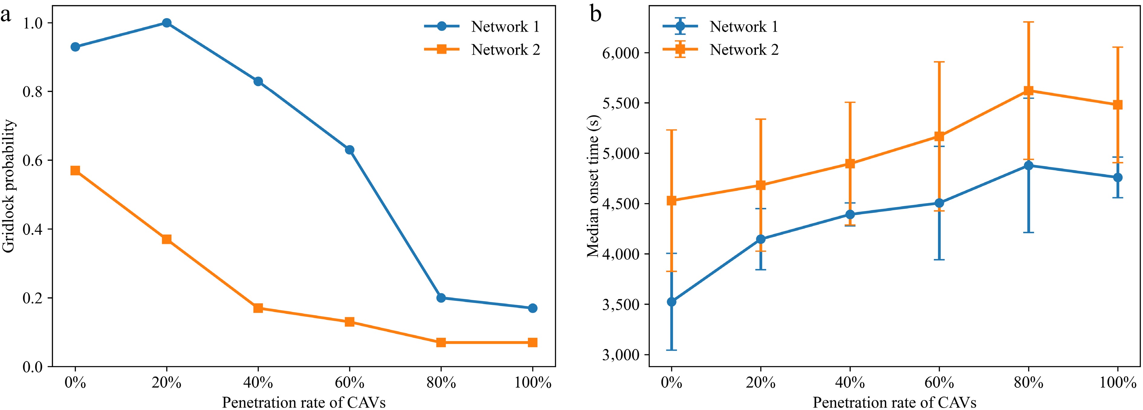
Figure 5. 

Gridlock probability and onset-time distribution under different CAV penetration rates. (a) Gridlock probability. (b) Median onset time.

This interpretation is further supported by the 95% confidence intervals of the empirical gridlock probabilities. In Network 1, the intervals for 0%, 20%, and 40% remain concentrated in a high-risk range, whereas the intervals for 80% and 100% fall into a much lower-risk range. The interval for 60% lies between these two groups, supporting its interpretation as a transition regime rather than a strict threshold. More importantly, the confidence intervals of 60% and 80% are clearly separated, while those of 40% and 60% still overlap, and those of 80% and 100% also overlap. This indicates that the most pronounced improvement in Network 1 is observed between 60% and 80%, whereas the additional gain beyond 80% is relatively limited.

By contrast, Network 2 exhibits the same overall tendency but substantially weaker gridlock risk. Its empirical probability declines from 0.57 at 0% penetration to 0.37, 0.17, 0.13, 0.07, and 0.07 as penetration rises from 20% to 100%, while the median onset time shifts later from 4,528.4 s to 4,681.9, 4,895.3, 5,167.8, 5,622.1, and 5,480.6 s. Compared with Network 1, the decline in Network 2 is much more gradual, and the confidence intervals of adjacent penetration scenarios overlap more substantially, especially from 40% onward. This suggests that the simplified arterial-only network does not exhibit an equally sharp segmentation of risk levels, but rather a smoother and more continuous decrease in vulnerability.

Figure 5 further highlights the contrast between the two network representations. Under the same normalized stress level, Network 1 remains highly susceptible to gridlock in low- and medium-penetration cases, whereas Network 2 appears considerably more stable throughout. In addition, the standard deviation of onset time remains non-negligible in several scenarios, especially in Network 1, indicating that even under identical demand and parameter settings, the exact onset of gridlock still depends on stochastic local interactions. Therefore, gridlock in oversaturated mixed traffic flow should be interpreted as a probabilistic outcome rather than as a purely deterministic threshold event.

Taken together, the results support two main conclusions. First, increasing CAV penetration generally postpones gridlock onset and reduces the probability of gridlock, but the improvement is nonlinear. In Network 1, the clearest reduction occurs between 60% and 80%, whereas the additional benefit beyond 80% is relatively small. Second, the full-network representation reveals substantially higher gridlock risk and earlier onset than the simplified benchmark network, implying that local and residential streets play an essential role in spillback interaction, bottleneck activation, and the realistic characterization of gridlock vulnerability.

Temporal deterioration and performance loss

Figure 6 shows the temporal evolution of network accumulation and trip completion flow. The upper panel indicates that, under low penetration rates, network accumulation rises more rapidly and reaches a higher level during the congested stage, implying that vehicles are stored in the network faster than they can be discharged. This pattern reflects the progressive buildup of queues and the strengthening of spillback interactions across links and intersections. By contrast, when the CAV penetration rate becomes higher, the increase in accumulation is generally slower, and the peak accumulation is lower, with the clearest separation from the low- and medium-penetration scenarios appearing in the high-penetration cases, especially at 80% and 100%. The lower panel of Fig. 6 provides a complementary interpretation from the perspective of trip completion flow. In low-penetration scenarios, the completion flow drops earlier and more sharply after congestion intensifies, indicating that the network gradually loses its discharge capability once queues begin to propagate. In higher-penetration scenarios, the decline in completion flow is generally milder and delayed, which implies that a larger proportion of CAVs helps preserve outflow stability and slows the transition from congestion to severe lock-up. Taken together, the two panels suggest that higher CAV penetration does not simply reduce congestion magnitude but also moderates the temporal deterioration process by suppressing excessive accumulation growth and sustaining the network's output capacity for a longer period.

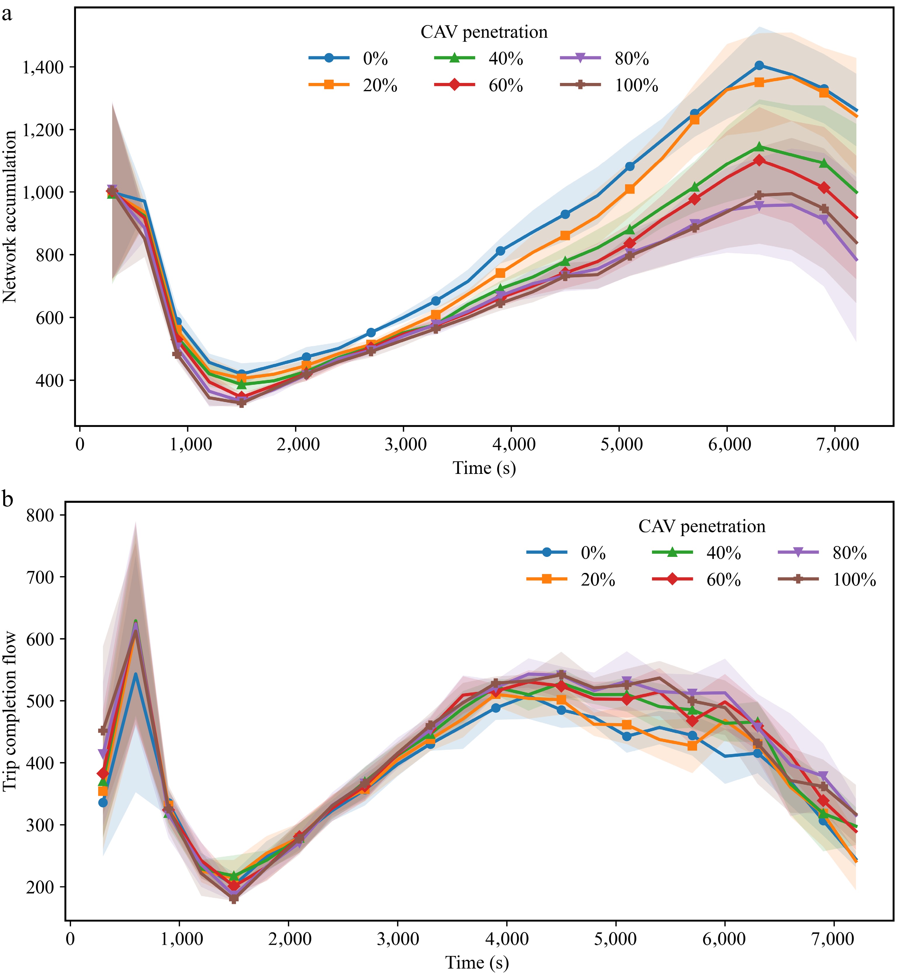
Figure 6. 

Temporal evolution of network accumulation and trip completion flow under different CAV penetration rates. (a) Temporal evolution of network accumulation. (b) Temporal evolution of trip completion flows.

The two panels jointly describe how the network transitions from high loading to reduced discharge performance under different penetration scenarios. The shaded regions represent the variability across multiple simulation runs with different random seeds. A larger shaded area indicates higher stochastic variability in network states, while a narrower band suggests more stable and consistent system behavior under the given penetration rate.

These two panels reflect the dynamic degradation of traffic efficiency and the cumulative system-wide delay under different mixed traffic compositions. Figure 7 further evaluates temporal deterioration from the perspectives of network mean speed and cumulative efficiency loss. The upper panel shows that network mean speed decreases much faster in low-penetration scenarios and remains at a lower level for a longer duration, which indicates a more severe and persistent degradation of traffic conditions throughout the network. In contrast, under higher penetration rates, the speed decline is more gradual, and the overall speed level remains comparatively higher, suggesting that the traffic state is less vulnerable to abrupt collapse. This difference becomes even clearer in the lower panel, where cumulative efficiency loss grows substantially faster under low-penetration conditions. Since this indicator captures the accumulated effect of high accumulation and speed degradation over time, its steep growth implies that low-penetration scenarios experience not only earlier deterioration but also more serious system-wide delay once congestion emerges. By comparison, high-penetration scenarios accumulate efficiency loss more slowly, meaning that the network can preserve its operational efficiency for a longer time even if congestion still develops. Therefore, Fig. 7 shows that the benefit of higher CAV penetration is reflected not only in postponing severe degradation but also in reducing the cumulative cost of congestion over the entire simulation horizon.

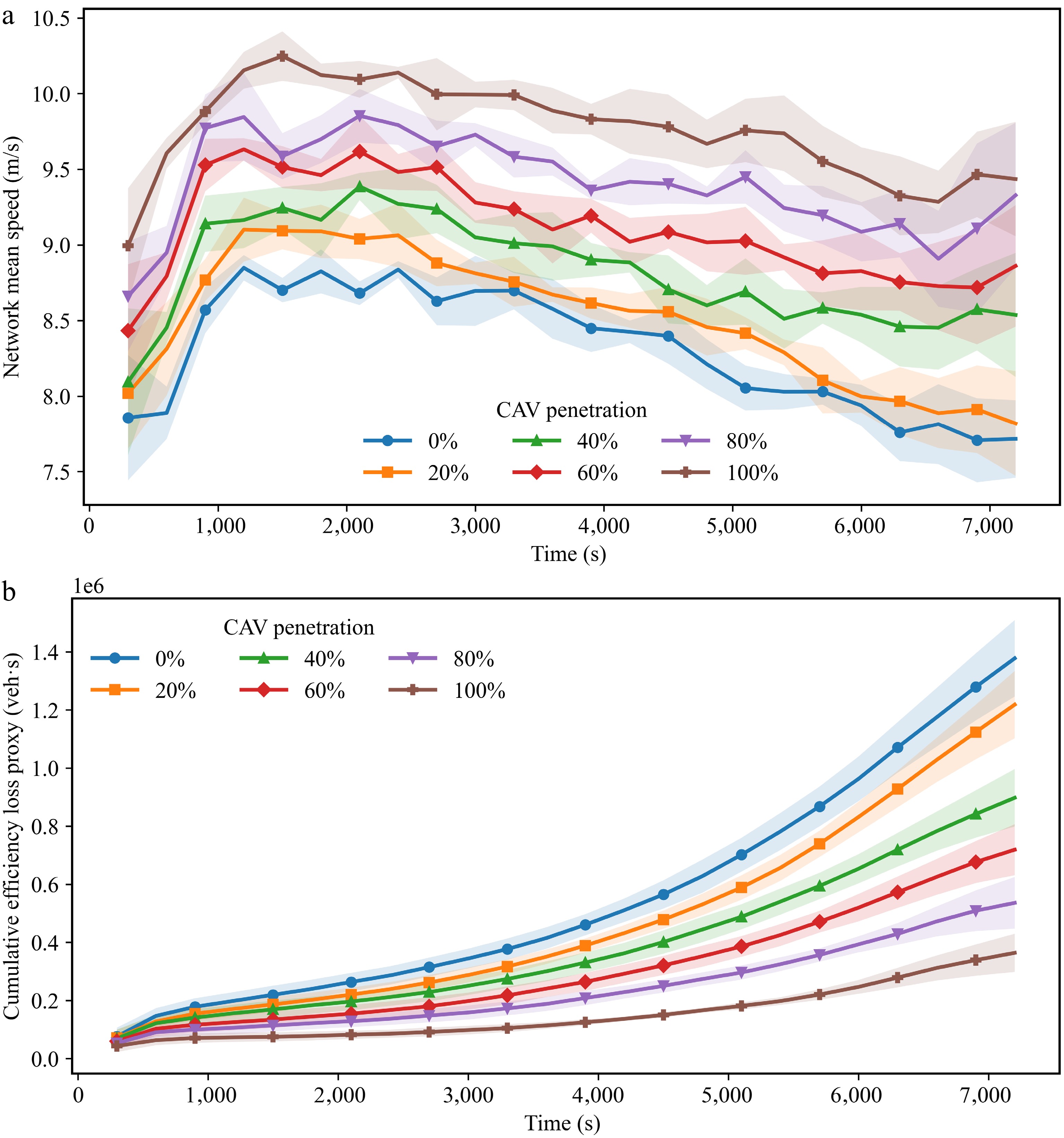
Figure 7. 

Temporal speed degradation and cumulative efficiency loss under different CAV penetration rates. (a) Network mean speed. (b) Cumulative efficiency loss.

Figure 8 summarizes these dynamic differences through two compact robustness indicators, namely the minimum network mean speed and the final trip completion flow. The first indicator reflects the worst operating state reached during the simulation. Lower values under low CAV penetration indicate that the network is more likely to enter an extremely degraded condition close to lock-up. The second indicator characterizes the residual discharge capability of the network at the terminal stage. Lower final completion flow means that, even near the end of the simulation, the system is still unable to recover effective outflow. In both respects, the results consistently show that low-penetration scenarios perform worse, whereas higher-penetration scenarios maintain a less severe worst-case condition and a stronger remaining flow output at the end. This implies that increasing the penetration rate of CAVs improves not only the transient evolution of congestion but also the robustness of the network in its worst and terminal states. At the same time, the variation across intermediate penetration rates suggests that the improvement is not perfectly monotonic, which is consistent with the stochastic and nonlinear nature of oversaturated mixed traffic flow.

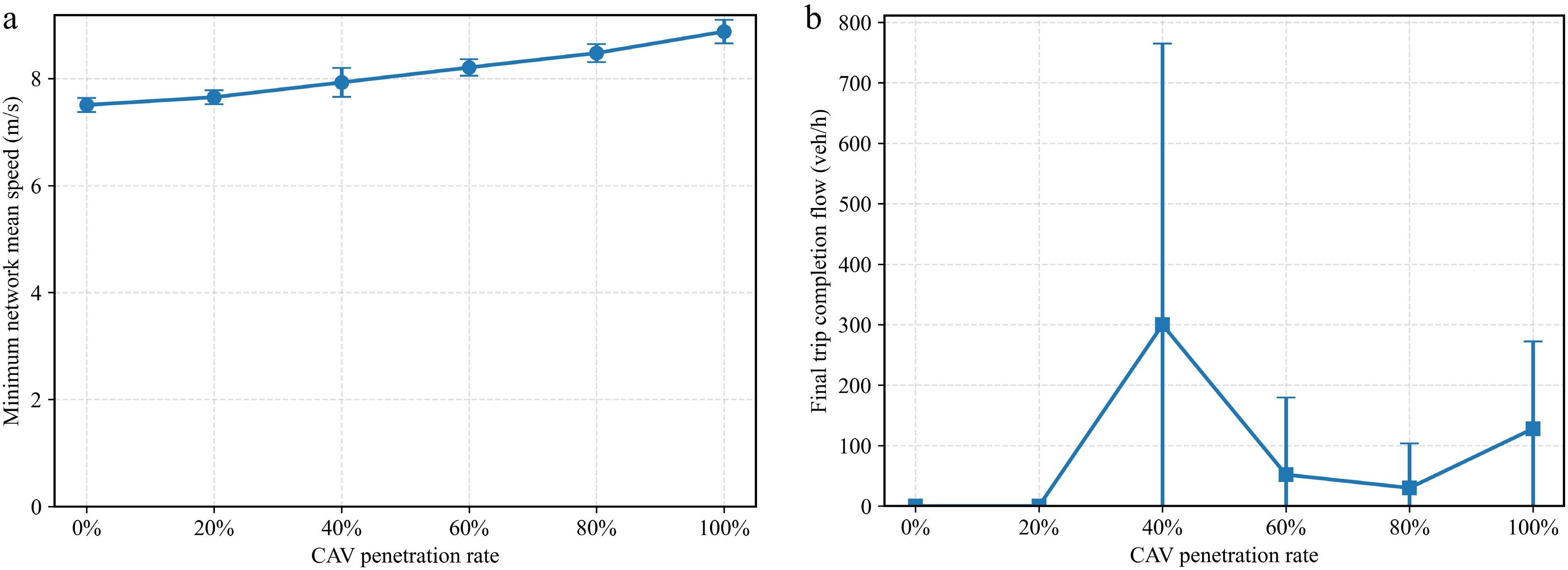
Figure 8. 

Robustness and terminal performance across penetration scenarios. (a) Minimum network mean speed. (b) Final trip completion flow.

Overall, we find that the effect of CAV penetration extends beyond gridlock onset itself. Higher penetration rates generally slow down accumulation growth, mitigate the drop in completion flow, maintain higher network speed, reduce cumulative efficiency loss, and improve both worst-case and terminal-stage performance. These results suggest that CAV penetration can enhance the temporal robustness of oversaturated urban networks. The improvement becomes more evident in the high-penetration regime, and in Network 1, the largest reduction in gridlock risk is observed between 60% and 80%, while the additional reduction beyond 80% is relatively limited.

Spatial concentration and propagation of gridlock

Because Network 2 exhibits substantially lower gridlock probability and much weaker persistent lock-up than Network 1, the detailed spatial concentration and propagation analysis is presented mainly for Network 1, where bottleneck-driven spreading can be observed more clearly.

Figure 9 provides a quantitative summary of the locations most closely associated with gridlock onset and persistent post-onset lock-up in Network 1. Figure 9a shows that the first gridlock onset event is not evenly distributed across all monitored intersections but is concentrated in a limited subset of recurrent bottlenecks. Although the dominant onset intersection varies across penetration scenarios, the first onset is repeatedly associated with only a few candidate locations, indicating that gridlock initiation is structurally localized rather than spatially random. In addition, the onset time is much earlier at 0% penetration than in the other scenarios, while most nonzero penetration cases show a delayed first onset. This is consistent with the occurrence statistics in Table 5 and Fig. 5, but it also suggests that increasing CAV penetration changes not only when gridlock emerges, but also which bottleneck is most likely to become active first.

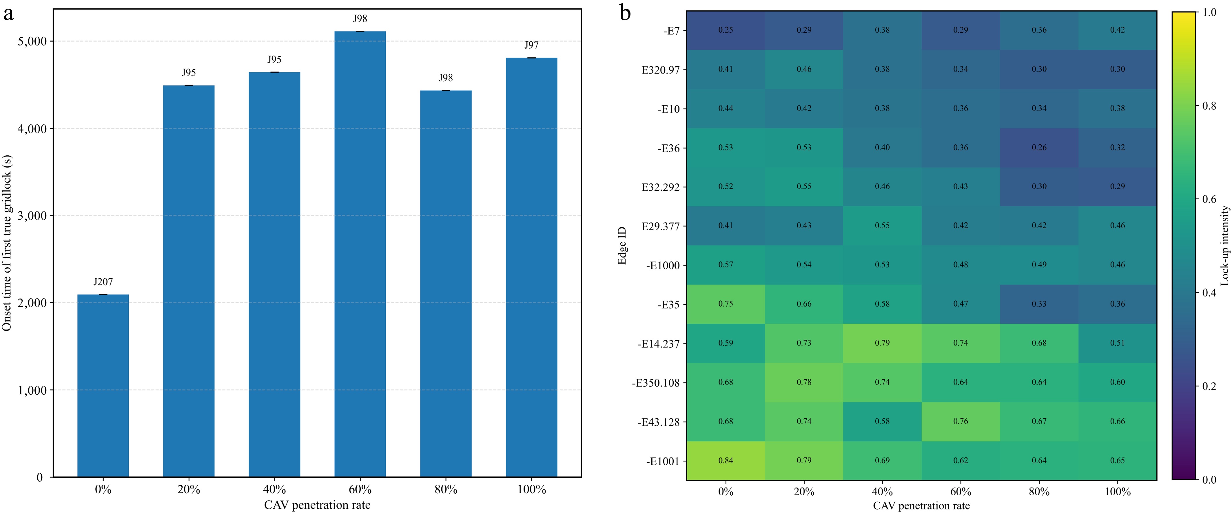
Figure 9. 

Spatial distribution of bottleneck probability and lock-up intensity in Network 1. (a) First detected gridlock onset time across penetration scenarios. (b) Lock-up intensity across penetration scenarios.

Figure 9b further characterizes the persistence of severe post-onset lock-up through the lock-up intensity of representative links. The results show that severe lock-up is concentrated on only a limited number of links, rather than being uniformly distributed across the network. Several links maintain relatively high lock-up intensity under low- and medium-penetration scenarios, indicating that they act as persistent carriers of spillback after gridlock onset. As the CAV penetration rate increases, the lock-up intensity on many of these links tends to decline, suggesting that higher CAV penetration can weaken the persistence of severe congestion on key road sections. However, this reduction is not strictly monotonic, since some intermediate- and high-penetration scenarios still retain noticeable lock-up on a few representative links. This again reflects the stochastic and nonlinear nature of oversaturated mixed traffic flow.

While Fig. 9 identifies the main high-risk intersections and links quantitatively, it does not by itself fully convey their spatial layout in the network. Figure 10 provides a spatial interpretation of the gridlock propagation patterns identified in Fig. 9 by mapping the affected intersections and links back onto the network. In these visualizations, deadlocked intersections are highlighted in orange, while links are classified into three categories according to their lock-up occurrence: repeated lock-up (red), occasional lock-up (yellow), and no lock-up (green). The figure therefore offers a qualitative representation of how congestion evolves and persists across different parts of the network under varying CAV penetration scenarios.

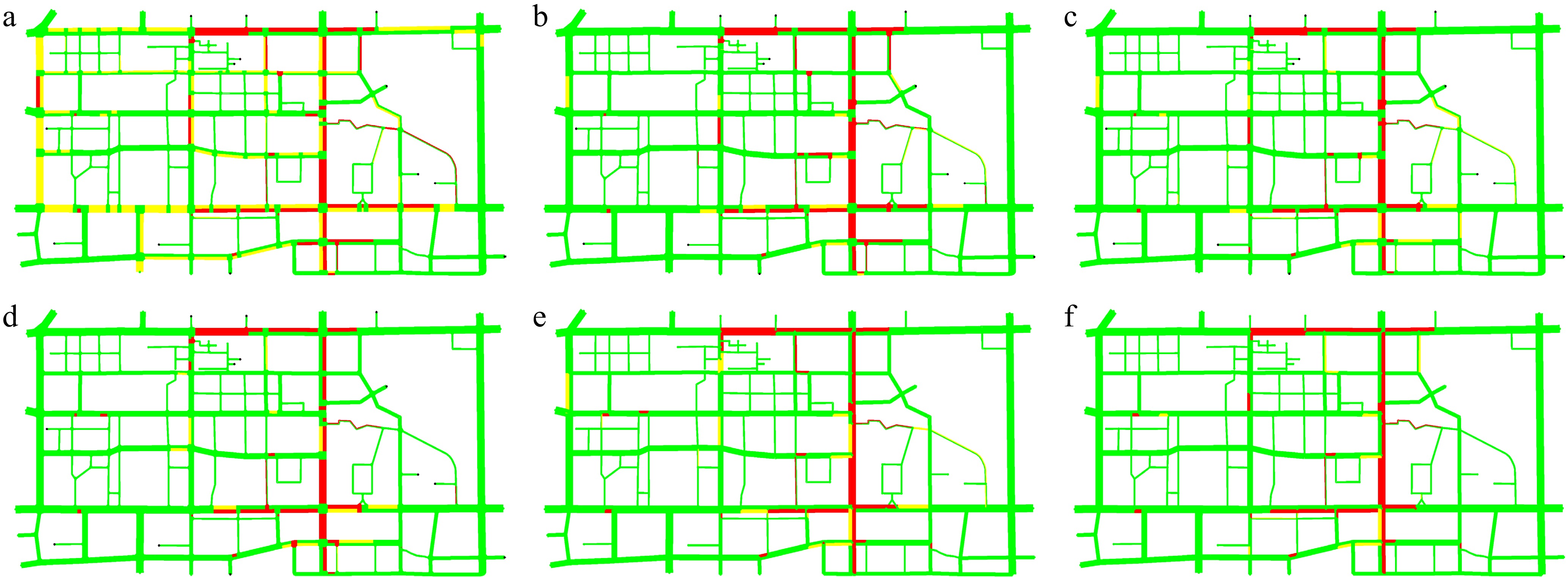
Figure 10. 

Representative spatiotemporal propagation of gridlock in Network 1. (a) Gridlock propagation at 0% CAV penetration. (b) Gridlock propagation at 20% CAV penetration. (c) Gridlock propagation at 40% CAV penetration. (d) Gridlock propagation at 60% CAV penetration. (e) Gridlock propagation at 80% CAV penetration. (f) Gridlock propagation at 100% CAV penetration.

At low penetration levels (0% and 20%), gridlock emerges relatively early and spreads over a broad spatial range. Multiple adjacent arterial links and intersections enter persistent deadlock states, forming extended connected regions of severe congestion. This indicates that once local bottlenecks are activated, spillback interactions quickly propagate along major corridors, leading to large-scale network degradation. At intermediate penetration levels (40% and 60%), the overall extent of severe lock-up is reduced compared with the lowest-penetration cases, but congestion remains clearly concentrated along several key arterial sections. The propagation pattern becomes less extensive but still exhibits corridor-based clustering, suggesting that the underlying bottleneck-driven mechanism remains active, although partially mitigated. At high penetration levels (80% and 100%), the spatial extent of gridlock is significantly constrained. Severe lock-up is largely confined to a small number of localized regions, and most links remain in non-lock-up or weakly affected states. This indicates that higher CAV penetration can effectively limit the spatial spread of congestion, even though localized bottlenecks may still persist.

Taken together, Figs 9 and 10 suggest that gridlock in Network 1 follows a bottleneck-driven propagation mechanism. Gridlock is first triggered at a few structurally vulnerable intersections, then persists on a limited number of key links, and finally spreads along major arterial corridors through spillback interactions. Higher CAV penetration does not remove this mechanism entirely, but it generally delays onset, weakens post-onset lock-up persistence, and reduces the spatial extent of severe propagation. Therefore, the spatial results indicate that mitigating gridlock in oversaturated mixed traffic requires not only increasing CAV penetration but also identifying and managing the limited set of bottleneck intersections and road sections that dominate network-wide deterioration.

MFD characteristics

Figure 11 compares the MFD patterns of Network 1 and Network 2 under different CAV penetration rates in the accumulation–trip-completion-flow plane. In both network representations, the observed state points exhibit a recognizable macroscopic relationship: when accumulation is relatively low, trip completion flow increases with network loading, whereas under heavier loading, the system gradually departs from this favorable regime. This confirms that both networks operate under a strongly unstable, oversaturated condition and that the deterioration observed in the microscopic simulations is also reflected in the macroscopic state evolution.

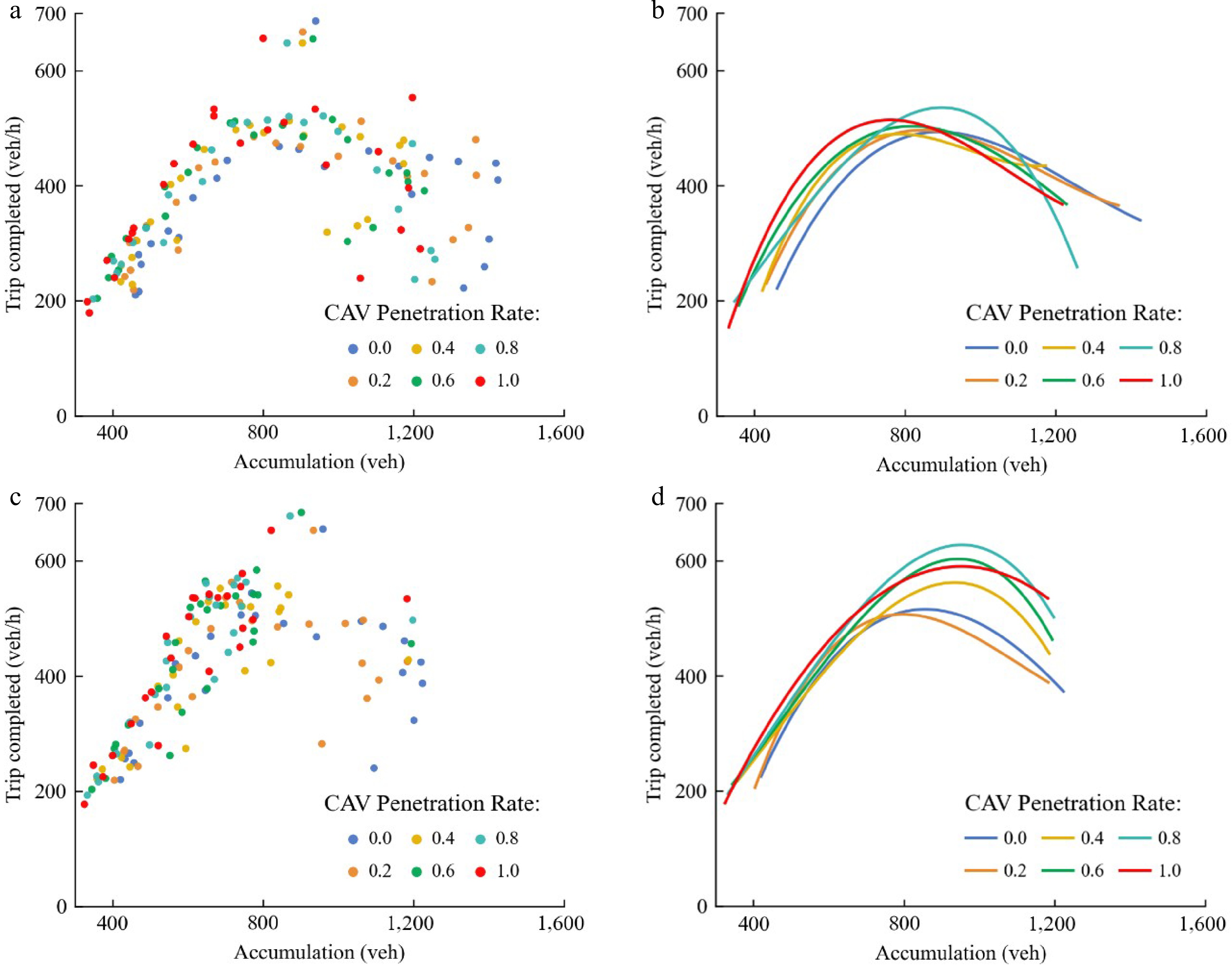
Figure 11. 

MFD trajectories and fitted curves of Network 1 and Network 2 under the same loading framework. (a) MFD trajectories in Network 1. (b) Fitted curve in Network 1. (c) MFD trajectories in Network 2. (d) Fitted curve in Network 2.

However, the two network representations show substantially different MFD characteristics. In Network 1, the state points are much more scattered, and the congested branch extends over a much wider accumulation range, especially under low and medium CAV penetration rates. In particular, some scenarios exhibit a long post-peak branch in which accumulation continues to rise while trip completion flow declines markedly. This pattern indicates severe discharge deterioration after congestion develops and suggests that the full network is strongly affected by local storage limitations, branch-road spillback, and bottleneck interactions. By contrast, Network 2 exhibits a much more compact point cloud and a smoother fitted envelope. Its state evolution remains concentrated within a narrower accumulation range, and the decline after the peak is much weaker. This implies that the simplified arterial-only representation suppresses part of the congestion heterogeneity and presents a more stable-looking macroscopic pattern.

The influence of CAV penetration is also different in the two networks. In Network 1, lower penetration scenarios are associated with broader scatter and more pronounced post-peak deterioration, while higher penetration scenarios tend to remain concentrated in a lower-accumulation and higher-completion-flow region. This suggests that increasing CAV penetration helps restrain excessive vehicle storage and mitigates the collapse of network discharge capacity. In Network 2, the fitted curves under different penetration rates are more regular and remain relatively close to one another in shape. The main effect of increasing penetration is therefore reflected more in a moderate upward or outward shift of the macroscopic envelope, rather than in a sharp reduction of collapse-like behavior. This difference further indicates that the apparent benefit of CAV penetration depends not only on traffic composition but also on how the network itself is represented.

The fitted curves in Fig. 11 should be interpreted only as descriptive summaries of the overall macroscopic envelopes. For Network 1 in particular, the larger scatter means that no single fitted curve can fully capture the full variability of congestion evolution once the system enters the congested regime. Nevertheless, the contrast between the two networks is informative: the full network reveals stronger heterogeneity, larger uncertainty, and more pronounced post-peak degradation, whereas the simplified network produces a smoother but more optimistic picture of network performance. Therefore, the MFD comparison supports the view that excluding local and residential streets may underestimate effective capacity constraints and gridlock-related vulnerability in heterogeneous urban road networks.

This study developed a macro–micro coupled framework to investigate gridlock risks in oversaturated mixed traffic flow on heterogeneous urban road networks. By combining microscopic simulation with MFD-based macroscopic interpretation, the study examined how different CAV penetration rates influence gridlock occurrence, temporal deterioration, and spatial propagation. Two network representations were considered: a full network including residential and branch roads, and a simplified arterial-only benchmark network. The results show that gridlock under oversaturated demand is inherently stochastic, but still exhibits clear statistical regularities with respect to traffic composition and network structure. In general, increasing the CAV penetration rate reduces gridlock probability and delays gridlock onset, although this improvement is not strictly monotonic across all scenarios.

The analysis further shows that CAV penetration affects not only whether gridlock occurs, but also how severely the network deteriorates once congestion emerges. Low-penetration scenarios are characterized by faster accumulation growth, earlier decline in trip completion flow, lower network mean speed, and greater cumulative efficiency loss. Spatially, gridlock is concentrated at a limited number of critical intersections and arterial links, and then propagates outward through spillback interactions. Higher CAV penetration generally weakens this bottleneck-driven propagation process by postponing onset, reducing lock-up persistence on key links, and shrinking the spatial extent of severe congestion. The results suggest that the mitigation of gridlock risk becomes most evident in the high-penetration regime, especially between 60% and 80% in the full-network scenario, whereas low- and medium-penetration scenarios remain much more vulnerable to instability. The identified gridlock-risk indicators can also provide practical guidance for spatial traffic intervention. Intersections with recurrent high gridlock probability can be treated as priority nodes for signal-control adjustment and queue spillback monitoring, while links with high post-onset lock-up intensity can be regarded as critical sections for storage-capacity monitoring and localized congestion mitigation. Under low CAV penetration, traffic management should focus on preventing early activation of bottleneck intersections, especially at arterial–branch connections where spillback may interfere with arterial discharge. Under high CAV penetration, the control emphasis may shift toward maintaining residual discharge capacity and preventing localized lock-up from expanding into corridor-level congestion. These implications do not constitute a complete control strategy, but they provide a direct link between gridlock-risk identification and potential measures such as dynamic signal management, network partitioning, and perimeter flow regulation.

Another important finding is that network representation strongly influences the interpretation of congestion risk. Compared with the simplified arterial-only network, the full network reveals higher gridlock probability, earlier onset, stronger bottleneck concentration, a wider and more scattered congested branch in the MFD, and more pronounced post-peak discharge deterioration. This indicates that excluding residential and branch roads may underestimate effective capacity constraints and mask local spillback interactions that are essential to gridlock formation. Therefore, evaluating oversaturated mixed traffic flow requires not only attention to CAV penetration but also explicit consideration of fine-grained local structures and critical bottleneck corridors. This study adopts a fixed 90-s cycle length with a standard four-phase signal plan to ensure controlled comparison across scenarios. However, in real heterogeneous networks, lower-level roads may have shorter signal cycles, weak signal control, or no signal control. Therefore, future work should further develop road-class-specific gridlock detection thresholds and examine how variable signal cycles and adaptive phase settings affect bottleneck activation and gridlock formation. In addition, several modeling configurations, such as the presence of central medians, the setting of U-turn locations, and channelization at intersections, may differ from real-world conditions. Moreover, our analysis is based solely on SUMO simulations^[31], and the adopted IDM and CACC parameters are literature-based baseline settings rather than site-specific calibration results under extremely high-density heterogeneous network conditions. Future work should further examine the sensitivity of key behavioral parameters, such as desired time gap, standstill distance, reaction time, and CACC control gains, using additional simulation platforms, alternative car-following models, and observed high-density mixed-traffic data^[32].