


-
According to statistics, as of 2021, there are 723 chemical parks in China, including 75 at the national level and 648 at the provincial level and below, the categories of hazardous chemicals in China announced by the emergency management department are 2,828[1]. There are great hidden dangers in the production, use, transportation and storage of hazardous chemicals. More and more chemical parks are also accompanied by more and more accidents, 5,207 hazardous chemical leakage accidents occurred in China from 2009 to 2018[2]. Accidents are often accompanied by leakage, fire and explosion, resulting in the atmospheric diffusion of hazardous chemicals, poisoning accidents and environmental pollution, which is of great social harm. Cao et al. selected 780 environmental pollution accidents of hazardous chemicals with strong representativeness, and the results showed that the environmental pollution accidents caused by leakage diffusion were the most frequent compared to fire and explosion, accounting for 53.9% of the total accidents[3]. For example, on August 12, 2015, an explosion at Ruihai in Tianjin Binhai New District spread at least 129 chemicals to the nearby area, killing 165 people, leaving 8 missing and 798 injured, and causing direct economic losses of 6.866 billion RMB; On March 21, 2019, a particularly significant explosion occurred at Tianjiayi Chemical Co., Ltd. in Xiangshui County, Jiangsu Province, in which aniline and ammonia nitrogen in the air, soil and water within 4 km of the explosion site were severely exceeded, and the diffused chlorine gas caused more than 30 people to be poisoned and affected 16 surrounding enterprises, resulting in a total of 78 deaths, and direct economic losses of 1.986 billion RMB; Outside of China, on December 3, 1984, a leakage of methyl isocyanate from the Union Carbide pesticide plant in India caused a total of 6,495 deaths, 125,000 poisonings, and 50,000 lifetime victims, making it a major tragedy in the world’s industrial history; On August 31, 2017, a peroxide leakage at the Arkema chemical plant in Texas, USA, caused 21 people to be poisoned by the spreading gas and evacuated residents within 1.5 miles of the site[4]. Table 1 lists some typical atmospheric dispersion events of accidental release that occurred from 2014 to present.
Table 1. Typical atmospheric dispersion events of accidental release.
Time Accident Consequences of the accident 2014.01.01 Hydrogen sulfide poisoning accident of Shandong Binhua Bingyang Combustion Chemical Co., Ltd, in China It caused a poisoning accident, resulting in 4 deaths, 3 injuries and direct economic loss of 5.36 million RMB 2015.12.17 Sulfur dioxide leakage accident of Excel Industries in India It caused 1 death and 4 people were poisoned and resuscitated 2016.01.09 Hydrogen fluoride leakage poisoning accident of Weifang Changxing Chemical Co., Ltd, in China It caused a poisoning accident, resulting in 3 deaths and 1 injury 2016.06.27 Explosion accident of pascagula gas plant in Mississippi, USA Surrounding residents were evacuated and the gas plant was closed for more than 6 months 2017.05.13 Chlorine gas leakage poisoning accident of Lixing Special Rubber Co., Ltd, in China It resulted in 2 deaths and 25 hospital admissions 2017.08.31 Chemical plant explosion in Texas, USA It resulted in the poisoning of 21 people and the evacuation of residents within a 1.5-mile radius of the accident site 2018.11.28 Vinyl chloride leakage and deflagration accident of Shenghua chemical company of China National Chemical Corporation in China It left 24 people dead and 21 injured 2019.04.02 Isobutylene leakage explosion at KMCO chemical plant in Crosby, Texas, USA. It resulted in 1 death, 2 people were seriously burned and at least 30 other workers were injured to varying degrees 2019.04.15 Poisoning accident of Qilu Tianhe Huishi Pharmaceutical Co., Ltd. in China It caused 10 deaths and 12 injuries, resulting in direct economic losses of 18.67 million RMB 2019.06.21 Fluorinated acid alkylation unit explosion at Philadelphia energy solutions corporation refinery in USA Smoke from the explosion covered much of downtown Philadelphia and South Philadelphia, causing minor injuries to 5 people 2020.05.07 Styrene leakage accident at LG Polymers Ltd. in India It caused 13 deaths and more than 5,000 people felt unwell to varying degrees 2021.04.21 Poisoning accident of Heilongjiang Kelunda Technology Co., Ltd., in China It resulted in 4 deaths and 6 toxic reactions The above-mentioned accidents have caused serious casualties and property loss. As a result of this situation, it is of vital importance to focus on the study of hazardous chemical leakage and diffusion accidents. To be more specific, it is necessary to predict the diffusion range of accidents quickly and accurately. This act can serve as a guide for emergency responders, providing key information for better evacuation actions and remedy for accidents. This paper introduces current main smoke dispersion prediction models, which are divided into three categories. Besides, each model is analyzed to summarize both advantages and disadvantages. Moreover, current study status of identification of fire and smoke have been reviewed in terms of atmospheric diffusion prediction model based on computer vision. And finally, the future development trend of prediction of atmospheric diffusion of hazardous chemicals has been proposed.
-
Both the dispersions of hazardous chemical gas and fumes due to accidental release in the atmosphere are affected by various factors such as wind speed, wind direction, atmospheric stability, release rate, release temperature, topography, obstacles and chemical reactions. Generally, the atmospheric dispersion is a temporal variation, but sometimes the gas and fumes can stay for a long time without dispersion[5], which is a multi-scale and complex process. After the accidental release of hazardous chemicals due to leakage, fire and explosion, gas or fume clouds can be formed in the atmosphere. For the gaseous hazardous chemical being flammable and explosive, where its volume concentration in the formed gas clouds is trapped in the range of explosion limits, fire and explosion accidents can occur in case of an ignition, and then produce gas or fume waste. For toxic hazardous gas, its diffusion can poison people, animals and other living beings near the source of accident release. Last but not least, both the aforementioned dispersions of accidental release can cause damage to the atmospheric system. Especially, considering the atmospheric dispersion of hazardous chemicals attributed to their containers’ rupture, the related leakage can be classified into three categories based on material phase state, namely leakages of gas phase, liquid phase and gas-liquid phase. Or according to the flow status of hazardous chemicals from containers, the corresponding leakages can be treated as continuous and transient ones. The continuous leakage refers to continuous source or release time longer than or equal to diffusion time; while transient leakage refers to leakage where the release time is much shorter than diffusion time. Herein, on the basis of previous research[6,7], the hazardous chemical leakage and its hazards are analyzed, and the entire process of accidental leakage is accompanied by diffusion, as shown in Fig. 1.
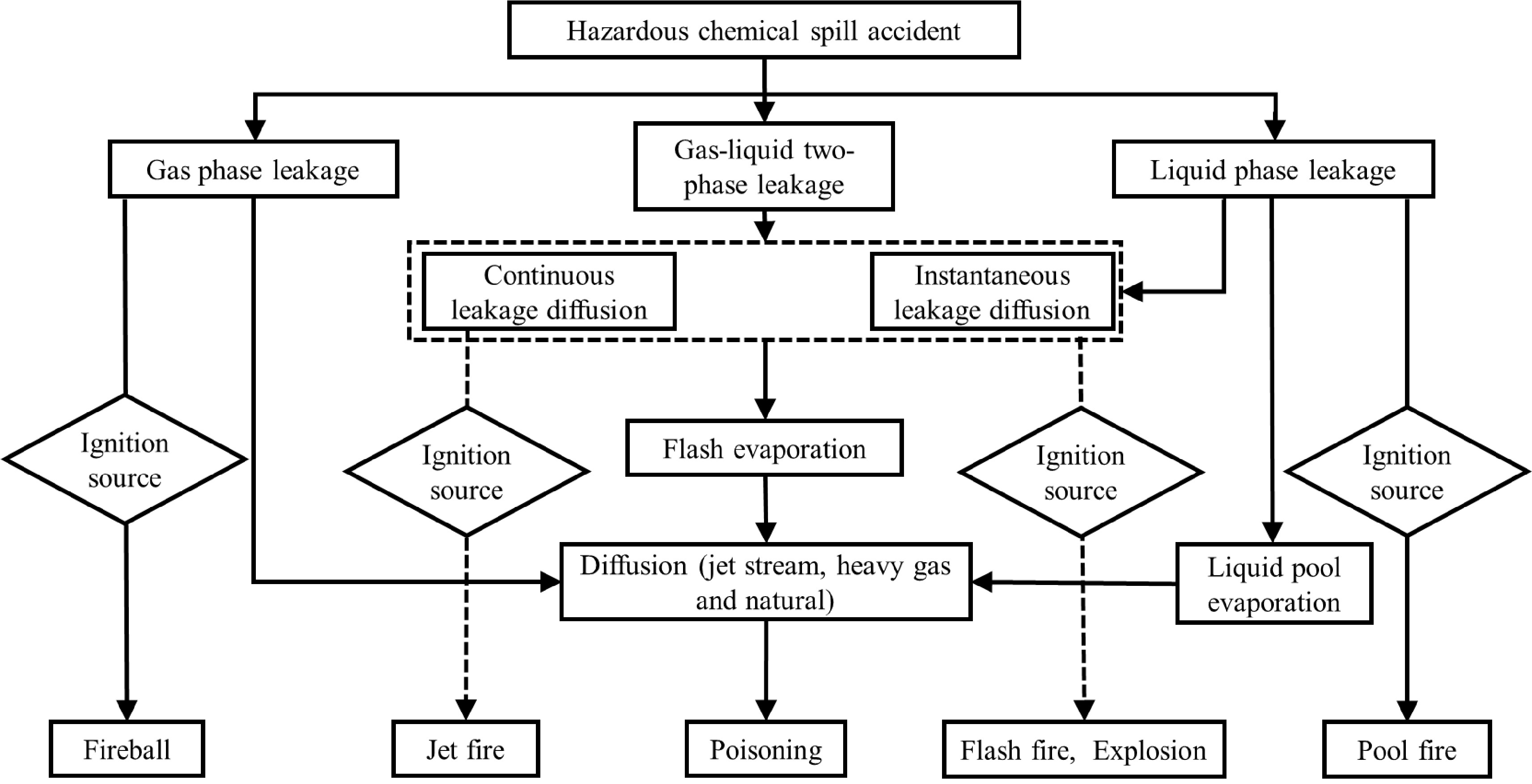
Figure 1.
Analysis of hazardous chemical accidents and their outcomes.
The impact range of hazardous chemical gas and fume dispersion is related to the leakage mechanism, dispersion characteristics and accident type, usually considering only the near-ground situation, spreading a few hundred meters or thousands of meters in the horizontal direction, and extending over time scales ranging from minutes to hundreds of years. Depending on the temporal and spatial span of dispersion, they can be divided into five categories:
(1) Small-scale diffusion: typical spatial span from 0 to 100 m, with time span ranging from minutes to hours.
(2) Urban-scale diffusion: also known as local-scale diffusion, with a typical spatial span of 100 to 10,000 m and a time span ranging from a few hours to a few days.
(3) Mesoscale diffusion: also known as regional-scale diffusion, with a typical spatial span of 10-100 km and a time span ranging from a few days to a few months.
(4) Meteorological-scale diffusion: refers to the movement of the entire meteorological system, with a typical spatial span of 100 to 1000 km and a time span of months, quarters or even years.
(5) Global-scale dispersion: typical spatial span is more than 5000 km, and the time span ranges from a decade to a century.
Based on the specific density of the hazardous gas relative to the air, it can be divided into three categories:
(1) Light gas (buoyancy) diffusion: lighter than air and can float.
(2) Neutral gas (natural gas, passive) diffusion: when the density ratio between hazardous gas and the average value of air is 0.9 to 1.1 times, the gas is called a neutral gas and will fuse with the air quickly.
(3) Heavy gas diffusion: When the density ratio between hazardous gas and the average value of air is greater than 1.1 times, or when the molecular weight is less than air. But due to the low temperature, the gas condenses into liquid droplets, this diffusion also belongs to heavy gas diffusion, which mostly flows along the ground. Heavy gas diffusion is most common in chemical production accidents and consists of four stages: heavy gas cloud deposition, air entrainment, cloud heating and transition to non-heavy gas clouds[8].
Inversion problem of leakage source parameters
-
In actual hazardous chemical accidents, the use of atmospheric dispersion prediction models or sensors only gather information on the concentration of hazardous chemicals, but not on the location and intensity of the leakage source, so it is necessary to invert the parameters of the leakage source. Leakage source parameter inversion relies on the concentration parameters obtained from the downwind, combined with the atmospheric dispersion model, to inverse the intensity information of the leakage source, and the solution process can be divided into deterministic method and probabilistic stochastic method.
The deterministic method can be divided into two categories, one is direct inversion, the parameters obtained from the detection and simulation of the least squares solution, and the use of the regularization method to transform the pathological characteristics of the least squares problem. But this solution method is only applicable to the Gaussian model and the real leakage scenario is complex and variable, so the direct inversion method is not practical. Another is optimization inversion, which is the use of optimization algorithms to minimize the difference between monitoring data and simulation data, and constantly optimize the location of the leakage source, to achieve the location of the leakage source. According to the different optimization methods used, they can be divided into: gradient methods (finding the derivative of the objective function, such as Newton’s method, conjugate gradient method), direct optimization methods (using only the value of the objective function without requiring the derivative, such as NM simplex method, pattern search method), intelligent optimization methods (with stochastic search capability, such as simulated annealing, genetic algorithms) and hybrid optimization methods. Lushi et al. used the linear least squares indirect optimization method to estimate the emission rate of the leakage source inversely by measuring the ground deposition of the material[9]. The Swarm intelligent optimization algorithm is less dependent on the initial value, Ma et al. compared particle swarm optimization algorithm, ant colony algorithm and firefly algorithm, and proposed an intelligent optimization method based on optimal correlation matching of concentration distribution, which takes into account the influence of atmospheric conditions and noisy data on the accuracy of the algorithm to improve the calculation of the leakage source location efficiency[10]. Qiu et al. used artificial neural networks for atmosphere diffusion simulation and used the expectation-maximization-based particle swarm optimization algorithm for inversion, which effectively accelerated the convergence process, but the prediction results beyond the training range were not accurate enough[11].
Probabilistic stochastic methods treat the leakage source parameters to be solved as random variables. The common methods are minimum relative entropy, statistical induction, and Bayesian inference methods. Among them, Bayesian inference methods are the most common probabilistic stochastic methods for solving such inverse problems with leakage source parameters. The method assumes that the leakage source parameters obey a priori distribution (generally Gaussian distribution), combines the detection data, calculates the posterior distribution of the parameters based on Bayesian theory, and then uses methods such as Monte Carlo sampling or Markov chain Monte Carlo sampling to calculate the estimated values of the parameters. Yee used Bayesian probability theory to derive the number of sources and the posterior probability density function for each source parameter (e.g., location, leakage rate, release time, and duration), and then established a mapping between the multi-source distribution and the measured concentrations of the detector array via a positive-time Lagrangian stochastic model[12]. Keats et al. used a Markov Chain Monte Carlo method to sample the posterior distribution of the source parameters and verified the feasibility of the method for the problem of inversion of highly disturbed flow fields in urban environments[13]. Iovino et al. counted the number of sources in an Italian southern city (about 32,000 inhabitants) of medium-sized cities for benzene, toluene, ethylbenzene, and isomeric xylenes, verifying the validity of the statistical method for the inversion problem of leakage sources[14].
Model classification
-
The European Commission’s Model Assessment Group divided heavy gas diffusion models into three categories: the first category is the phenomenological model with a series of icons and simple statistical representations; the second category is intermediate models, including one-dimensional integral models based on box models and two-dimensional models based on shallow equations; and the third category is the three-dimensional hydrodynamic model based on solving the Navier-Stokes equations[15]. Yi et al. classified the existing atmospheric diffusion models into Computational Fluid Dynamics (CFD) models and probabilistic models[16]. Sun et al. classified the models into empirical models, engineering application models and research models according to the application characteristics of heavy atmospheric models[17]. In this paper, according to the different modeling principles, the existing atmospheric dispersion prediction models are classified into simplified-experience models, mechanism- and rule-driven models and data-driven models.
-
Among the casualties caused by hazardous chemicals, about 90% are related to heavy gas leakage, which causes about 99.05% of the total casualties[18]. In order to predict the spread of hazardous chemicals after gas leakage quickly and accurately, a large number of experimental studies have been carried out by previous researchers, which are mainly divided into two categories: field experiments and wind tunnel tests[19].
Field experiments simulate the situation of hazardous chemical leakage in a more realistic way, and restore the leakage volume, leakage rate, geographical environment and other factors of the leakage substance in equal proportion, so that the data obtained is real and reliable. The disadvantages of the field experiment are also obvious, including the high risk, huge cost, difficulty in repeating the experiment, limited by environmental conditions, and the need for follow-up treatment after the experiment. Some special experimental phenomena can only be observed through field experiments, such as the LNG experiments conducted in California in 1980, where bifurcations in the front end of the diffused gas can be seen. Table 2 lists the most well known foreign field experiments.
Table 2. Famous foreign experiments on diffusion of toxic gases[20].
Parameters Experiment Burro Coyote Desert
TortoiseGoldfish Maplin
SandsThorney
IslandThorney
IslandFladis Number of experiments 8 3 4 3 12 9 2 16 Test medium LNG LNG NH3 HF LNG Freon/N2 Freon/N2 NH3 Leakage source Boiling point heavy gases Boiling point heavy gases Two-phase heavy gases Two-phase heavy gases Boiling point heavy gases Heavy gases Heavy gases Two-phase heavy gases Total amount of release (t) 10.7−17.3 6.5−12.7 10−36.8 35−38 1−6.6 3.15−8.7 4.8 0.036−1.2 Release time (s) 79−190 65−98 126−381 125−360 60−360 Momentay 460 180−2,400 Release surface Water Water Sandy soil Sandy soil Water Sandy soil Sandy soil Sandy soil Surface roughness 0.0002 0.0002 0.003 0.003 0.0003 0.005−0.018 0.005−0.018 0.01 Atmospheric stability C−E C−D D−E D D D−F D−F E−F Farthest distance (m) 140−800 300−400 80 3,000 460−650 500−800 500−800 240 Year of experiment 1982 1983 1985 1987 1984 1985 1985 1993−1996 Wind tunnel tests are conducted by placing the flying vehicle and other object in a wind tunnel to study the atmospheric flow and its interaction with the object. Because wind tunnel tests are easy to use, efficient and safe, low cost and easy to control, some scholars at home and abroad have obtained a large number of conclusions through wind tunnel tests. Korgstad et al. simulated the dispersion of a hemispherical emission device during continuous leakage by wind tunnel tests and found that the plume passes through the building and forms a step horseshoe-shaped vortex, which will greatly reduce the value of the atmospheric concentration at the building wall, and the degree of reduction depends on the height ratio of the plume to the model[21]. Liu explored the transient source, the diffusion characteristics of heavy gas plume, and the effect of fences and trees on the diffusion behavior through wind tunnel tests[22]. Li established a numerical calculation model for the diffusion of carbon dioxide two-phase clouds based on the principle of carbon dioxide leakage, designed wind tunnel tests to validate the model, and studied the distribution characteristics of the hazardous area after a liquid chlorine leakage accident in an urban environment based on the carbon dioxide diffusion model[23]. Xin et al. designed wind tunnel tests in a radius of 3 km at a scale of 1:1000, with a maximum vertical distance of 750 m in the whole experimental area, and compared the differences in mixed natural gas concentrations between CFD simulation results and wind tunnel experimental results at different distances from the leakage source, and discussed the effects of wind speed, wind direction, topography and their interactions on the natural gas dispersion process and hazard range[24]. However, wind tunnel tests are difficult to simulate diffusion under low turbulence conditions, and the diffusion behavior of heavy gas at low wind speeds is not well understood[19].
Many scholars have summarized the atmospheric diffusion prediction models for different diffusing substances and different scenarios after conducting a large number of field experiment and wind tunnel tests. These atmospheric diffusion models take the leakage source as the starting point, simplify the diffusion process, and use mathematical formulas to express the approximate diffusion range and concentration distribution of the leakage material, which are collectively referred to as atmospheric diffusion prediction models based on experience simplification in this paper. The more widely used ones are Gaussian model, Pasquill-Gifford model, Sutton model, BM model, box model, FEM3 model, etc. The empirical models applicable to neutral gas and light gas diffusion include the Gaussian model and the Sutton model, among others, and the models applicable to heavy atmospheric diffusion include image-only model, box model, FEM3 model, and shallow layer models. There are many models in this category, while the Gaussian model, Sutton model and Pasquill-Gifford model for neutral gas and light gas diffusion, and the Phenomenological Model, box model, FEM3 model and shallow model for heavy gas diffusion are introduced in this paper[25].
Gaussian plume model
-
The Gaussian model is suitable for the estimation of atmospheric dispersion along flat areas. The airflow in the atmospheric environment is relatively stable and uniform. The release gas diffuses and initially moves in the dominant wind direction, and the particle motion satisfies the normal Gaussian distribution. The basis of Gaussian model is the theory of turbulent diffusion gradients. Gradient theory uses Euler’s method to discuss the change in mass flux (concentration of pollutants) caused by turbulent motion at a fixed point in space, and the turbulent flux is proportional to the concentration gradient at that point. The Gaussian model includes the puff model and the plume model, which is only applicable to neutral gas with densities similar to air, and is one of the most widely used models at present[26]. The Gaussian plume model is commonly used to describe the stable concentrations of continuous release sources and is based on holding certain ideal conditions[27]. The model is established in a fixed space Eulerian coordinate system, and without considering the boundary conditions, the concentration calculation equation can be written as:
$\begin{split} C(x,y,z)=&\frac{Q}{2\pi i{\sigma }_{y}{\sigma }_{z}}\mathrm{e}\mathrm{x}\mathrm{p}\Bigg[-\frac{{y}^{2}}{{2\sigma }_{y}^{2}}\Bigg]\Bigg\{\mathrm{e}\mathrm{x}\mathrm{p}\Bigg[-\frac{{\left(z-H\right)}^{2}}{2{{\sigma }_{z}}^{2}}\Bigg]+\\&\mathrm{e}\mathrm{x}\mathrm{p}\Bigg[-\frac{{\left(z+H\right)}^{2}}{2{{\sigma }_{z}}^{2}}\Bigg]\Bigg\}\end{split} $ (1) where
$ C(x,y,z) $ $ (x,y,z) $ $ {\sigma }_{y} $ $ {\sigma }_{z} $ $ {\sigma }_{y} $ $ {\sigma }_{z} $ The assumptions of the Gaussian plume model are as follows:
(1) All variables do not change with time;
(2) It applies to the diffusion of a gas with a density similar to that of air (without taking into account the effect of gravity or buoyancy), and that no chemical reactions occur during the diffusion process;
(3) The properties of the diffusing gas are the same as those of air;
(4) Complete reflection without any absorption when the diffuse material reaches the ground.
(5) Turbulent diffusion in the downwind direction is negligible with respect to the shifting phase, which means that the model is only applicable to situations where the average wind speed is not less than 1 m/s;
(6) The x-axis of the coordinate system coincides with the flow direction, and the lateral velocity component V and the vertical velocity component W are zero;
(7) Assuming ground level.
The Gaussian plume model is simple and easy to use, but the results are often only used to roughly determine the extent of atmospheric dispersion, and is only applicable to calculate the concentration distribution of released substances within 10 km[20]. The Gaussian plume model needs to be valid under the above conditions, so there is a large error with the actual situation, and after correction, more complex scenarios can be calculated. For example, the Gaussian plume model was mostly applied to the prediction of atmospheric dispersion in plain areas, and He et al. added the terrain factor to the Gaussian plume model and analyzed the law of toxic atmospheric dispersion under four different terrains, which had certain reference value for toxic gaseous leakage accidents[28]. Liu improved the Gaussian plume model by using the ground reflection coefficient and correction coefficient, solved the objective function by using POS, and optimized the model parameters based on AFTOX monitoring data to improve the accuracy of inverse calculation of source intensity[29]. Lee used the Gaussian plume model to predict the smoke concentration in fire accidents[30].
Gaussian puff model
-
The Gaussian puff model assumes that the diffused atmosphere is composed of multiple instantaneous emission puffs, and the puff concentration obeys the Gaussian distribution. At the same time, the movement and diffusion of each puff are only affected by the wind speed and direction where the puff is located. The concentration at a certain point in the space is the accumulation of the concentrations of all puffs at that point. The Gaussian puff model is often used to describe the instantaneous concentrations of quantitative independent release sources, and can be capable of calculating atmospheric dispersion within 50 km in the horizontal direction due to the reduced requirement for leakage sources and wind fields. The Gaussian plume model uses the Lagrangian coordinate system in which the spatial location can be moved, and the concentration calculation equation can be written as:
$ \begin{split}C\left(x,y,z,t\right)=&\frac{M}{{\left(2\pi \right)}^{\frac{3}{2}}{\sigma }_{x}{\sigma }_{y}{\sigma }_{z}}\mathrm{exp}\left[-\left(\frac{{\left(x-ut\right)}^{2}}{2{{\sigma }_{x}}^{2}}\right)\right]\times\mathrm{exp}\left(-\frac{{y}^{2}}{2{{\sigma }_{y}}^{2}}\right)\times\\& \left\{\mathrm{exp}\left[-\frac{\left(z-H\right)}{2{{\sigma }_{z}}^{2}}\right]+\mathrm{e}\mathrm{x}\mathrm{p}\left[-\frac{{\left(z+H\right)}^{2}}{2{{\sigma }_{z}}^{2}}\right]\right\}\end{split} $ (2) Where, t is the diffusion time, in s; M is the total amount of leakage, in g; u is the average wind speed of the environment at the time of leakage, in m/s;
$ {\sigma }_{x} $ Sutton model
-
The Sutton model solves the distribution of all particles in space by studying the diffusion phenomenon of individual particles with mathematical and statistical methods, which is applicable to the problems of turbulent diffusion, large leakage and long leakage time. But the model does not compute the influence of gravity on the diffusion process, only applicable to light gas and neutral gas diffusion, dealing with the diffusion of combustible gas is also inaccurate. The accuracy of the model is poor, and the application is less widespread. Its concentration distribution calculation formula is:
$\begin{split} C\left(x,y,z\right)=&\frac{M}{\mathrm{\pi }{\sigma }_{y}{\sigma }_{z}u}\mathrm{e}\mathrm{x}\mathrm{p}\Bigg\{-\frac{{y}^{2}}{{{\sigma }_{y}}^{2}{x}^{2-n}}\Bigg[\exp\left[-\frac{{\left(z-H\right)}^{2}}{{{\sigma }_{z}}^{2}{x}^{2-n}}\right]+\\&\exp\left[\frac{{\left(z+H\right)}^{2}}{{{\sigma }_{y}}^{2}{x}^{2-n}}\right]\Bigg]\Bigg\}\end{split} $ (3) where n is related to weather conditions and is dimensionless, and the remaining parameters have the same meaning as above.
Pasquill-Gifford model
-
The Pasquill-Gifford model is one of Sutton’s derivative models, which is a dynamic simulation of non-heavy gas with stable wind speed in the plain on the basis of referring to the level of atmospheric stability. Depending on the given diffusion conditions, Pasquill-Gifford stability classes are classified as A–F, where A–C stands for unstable, D for neutral, and E–F for stable[32]. If the Pasquill-Gifford model is employed to predict atmospheric dispersion, the first step is to determine atmospheric stability level according to meteorological data, and then the corresponding σy and σz curves according to the stability can be selected (Tables 3 & 4).
Surface wind
speed (m/s)Daytime sunshine Nighttime conditions Strong Moderate Slight Thinly overcast or
> 4/8 low cloud< 3/8 cloud < 2 A A–B B F F 2–3 A–B B C E F 3–4 B B–C C D E 4–6 C C–D D D D > 6 C D D D D Table 4. Recommended Pasquill-Gifford model diffusion coefficient equation for plume dispersion (downwind distance x in m).
Pasquill-Gifford
stability rating$ {\mathit{\sigma }}_{\mathit{y}} $/m $ {\mathit{\sigma }}_{\mathit{z}} $/m Rural conditions A 0.22x(1 + 0.0001x)−1/2 0.20x B 0.16x(1 + 0.0001x)−1/2 0.12x C 0.11x(1 + 0.0001x)−1/2 0.08x(1 + 0.0002x)−1/2 D 0.08x(1 + 0.0001x)−1/2 0.06x(1 + 0.0015x)−1/2 E 0.06x(1 + 0.0001x)−1/2 0.03x(1 + 0.0003x)−1/2 F 0.04x(1 + 0.0001x)−1/2 0.016x(1 + 0.0003x)−1/2 City conditions A–B 0.32x(1 + 0.0004x)−1/2 0.24x(1 + 0.0001x)−1/2 C 0.22x(1 + 0.0004x)−1/2 0.02x D 0.16x(1 + 0.0004x)−1/2 0.14x(1 + 0.0003x)−1/2 E–F 0.11x(1 + 0.0004x)−1/2 0.08x(1 + 0.0015x)−1/2 Note: A–F are as defined in Table 3. The plume of a continuous steady-state source can be expressed as:
$\begin{split} C\left(x,y,z\right)=&\frac{Q}{\pi {\sigma }_{y}{\sigma }_{z}u}\mathrm{e}\mathrm{x}\mathrm{p}\left[-\left(\frac{{y}^{2}}{{2\sigma }_{y}^{2}}\right)\right]\times \Bigg\{\mathrm{e}\mathrm{x}\mathrm{p}\left[-\frac{1}{2}{\left(\frac{z-H}{{\sigma }_{z}}\right)}^{2}\right]+\\&\mathrm{e}\mathrm{x}\mathrm{p}\left[-\frac{1}{2}{\left(\frac{z+H}{{\sigma }_{z}}\right)}^{2}\right]\Bigg\} \end{split}$ (4) The smoke mass of a transient point source can be expressed by the equation:
$\begin{split} C\left(x,y,z\right)=&\frac{Q}{{\left(2\pi \right)}^{\frac{3}{2}}{\sigma }_{y}{\sigma }_{y}{\sigma }_{z}}\mathrm{e}\mathrm{x}\mathrm{p}\left[-\frac{1}{2}\left(\frac{{y}^{2}}{{\sigma }_{y}^{2}}\right)\right]\times \Bigg\{\mathrm{e}\mathrm{x}\mathrm{p}\left[-\frac{1}{2}{\left(\frac{z-H}{{\sigma }_{z}}\right)}^{2}\right]+\\&\mathrm{e}\mathrm{x}\mathrm{p}\left[-\frac{1}{2}{\left(\frac{z+H}{{\sigma }_{z}}\right)}^{2}\right]\Bigg\}\times \mathrm{e}\mathrm{x}\mathrm{p}\left[-\frac{1}{2}{\left(\frac{x-ut}{{\sigma }_{x}}\right)}^{2}\right]\end{split} $ (5) The meaning of the above formula parameters are the same as above.
The Pasquill-Gifford model is unconstrained in time and space, but requires appropriate boundary layer conditions and initial conditions, is subject to more human factors, and has poorer computational accuracy. Luo used information technology such as virtual reality and Internet technology combined with Gaussian model and Pasquill-Gifford model to construct a 3D simulation system for the digital park of chemical park[33].
Phenomenological model
-
The phenomenological model is what Britter and McQuaid used to connect the data in a dimensionless form and plot it as a curve and column graph with the data match on the basis of a large number of field experiments, and developed a heavy gas diffusion manual, also known as the BM model[5]. The phenomenological model describes the process of atmospheric diffusion with simple equations and column graphs, and the concentration at a point can be obtained by looking up in a table, which is easy to use, but the experimental results are not accurate and practical. Hanna et al. obtained some simple fitting equations by dimensionless processing of experimental data, which are correspond with the experimental data and can simulate the diffusion process of heavy gas release very well[34].
The heavy gas continuous leakage dispersion equation is:
$ \frac{{C}_{M}}{{C}_{0}}={f}_{c}\left[\frac{x}{{{(V}_{{C}_{0}}/U)}^{\frac{1}{2}}},\;\frac{{g}_{0}^{,}{V}_{{c}_{0}}^{\frac{1}{2}}}{{u}^{\frac{5}{2}}}\right] $ (6) The function is a universalized dimensionless function. Where,
$ {C}_{M} $ $ {C}_{0} $ $ {V}_{{C}_{0}} $ $ {g}_{0}^{,} $ The heavy gas transient leakage dispersion fitting equation is:
$ \frac{{C}_{M}}{{C}_{0}}={f}_{i}\left[\frac{x}{{{V}_{{i}_{0}}}^{\frac{1}{2}}},\;\frac{{g}^{\text{'}}{V}_{{i}_{0}}^{\frac{1}{3}}}{{u}^{2}}\right] $ (7) where
$ {V}_{{i}_{0}} $ Box model and similar model
-
The mixed dilution effect of a gas cloud in the initial stage occurs when it falls and spreads around, and the surrounding air enters from its periphery; in the later stage, due to the strong turbulence of the gas cloud, the surrounding air enters from the top. When the density of the gas cloud is diluted close to that of the atmosphere, atmospheric turbulence plays a dominant role, and then atmospheric diffusion begins. Ulden's heavy gas cloud experiment shows that the lateral diffusion parameter of the plume is four times that of neutral gas cloud, and the vertical diffusion parameter of the plume is 1/4 of that of a neutral gas cloud. This trend is called gravity settling. For the instantaneous release of heavy gas, Ulden proposed the concept of the box model[35]. The box model is used for heavy gas diffusion prediction, treating the heavy gas cloud as a cylinder, describing only the overall characteristics of the gas cloud without considering the detailed features, simpler than the Gaussian model, higher computational accuracy, and suitable for scenes with large accidents. The box model is based on three basic assumptions: (1) The heavy gas cloud is approximated as a cylinder with an initial height of half the radius; (2) The parameters such as temperature field and concentration field inside the heavy gas cloud obey uniform distribution; (3) The center of the cloud moves with a speed equal to the wind speed of the environment in which it is located. The basic equations of the box model are:
The radial expansion of the cloud mass is:
$ \frac{dR}{dt}={C}_{E}{\left({g'}L\right)}^{\frac{1}{2}} $ (8) The entrainment rate of air is:
$ \frac{dV}{dt}=\pi {R}^{2}{u}_{e}+2\pi RL{w}_{e} $ (9) where L is the cloud height, in m; R is the cloud radius, in m;
$ {u}_{e} $ $ {C}_{E} $ The box model includes the HEGADAS model, Cox and Carpenter model, Eidsvik model, Fay model, Germeles and Drake model, Piecknett model, Van Buijtenen model, and the Van Ukden model. Figure 2 shows the shape of the smoke plume of the HEGADAS model in the ideal state. Based on the box model, Jiang & Pan established a new type of model to describe the diffusion process of heavy gas leakage, which was simple in form and fast in operation speed, and it worked well in simulating the Throney Island Field Trials series of tests, but the simulation of heavy gas diffusion in other occasions have large deviations. And some properties of the model itself will bring an error, such as the model makes many assumptions, the error caused by the measurement components and human factors, and insufficient research on the mechanism of heavy gas diffusion[36].
Figure 2.
HEGADAS model plume shape in the ideal state [37].
The similar model is an improvement of the box model, which mainly includes the HEGADAS model and the model developed based on HEGADAS, which takes into account the internal velocity and concentration distribution of the gas cloud in diffusion[38]. In the box model, it is assumed that the inside of the gas cloud obeys a uniform concentration distribution and velocity distribution, while the similarity model further assumes that there is a certain distribution of concentration and velocity inside the gas cloud, such as similarity distribution or power function distribution. Another difference is that the similar model uses turbulent diffusion coefficients rather than the air entrainment rate to simulate the air percolation and mixing phenomena.
Shallow layer model
-
The shallow layer model is obtained based on a generalization of the shallow theory (shallow water equation)[39], where the controlling equation for heavy atmospheric diffusion is simplified to describe its physical processes, assuming that the lateral dimensions of heavy gas clouds are much larger than the vertical dimensions, and that the pressure distribution within the main body of the gas cloud can be described by hydrostatic theory, with special phenomena occurring only at the front edge of the gas cloud[17], and this assumption is applicable inside the whole gas cloud. It uses thickness-averaged variables to characterize the flow field, which is applicable to complex terrain. The mathematical equations of the shallow layer model are:
$ \frac{\partial h}{\partial t}+\frac{\partial h\mu }{\partial x}+\frac{\partial hv}{\partial y}=0 $ (10) $ \frac{\partial h\rho \mu }{\partial t}+\frac{{\partial h\rho \mu }^{2}}{\partial x}+\frac{\partial h\rho \mu v}{\partial y}+\frac{\partial }{\partial x}\left[\frac{1}{2}\mathrm{g}(\rho -{\rho }_{a}){\mathrm{h}}^{2}\right]=0$ (11) $ \frac{\partial h\rho v}{\partial t}+\frac{\partial h\rho \mu v}{\partial x}+\frac{{\partial h\rho v}^{2}}{\partial y}+\frac{\partial }{\partial y}\left[\frac{1}{2}\mathrm{g}(\mathrm{\rho }-{\mathrm{\rho }}_{a}){h}^{2}\right]=0 $ (12) where ρ is the stable density, in kg/m3; h is the depth of water flow, in m; μ is the velocity of water flow in m/s; and
$ {\rho }_{a} $ The shallow layer model can be divided into one-dimensional models and two-dimensional models. One-dimensional models use only one variable to describe the effect of spatial location on concentration, and all other attributes are approximated as average distribution in space, and the accuracy is poor when solving for complex terrain and with obstacles, and common one-dimensional models are SLAB and DISPLAY-I. The SLAB model[40] was developed by the Lawrence Livermore National Laboratory, (University of California, USA) which can be used to calculate four types of surface evaporation pools, horizontal jetting on overhead, vertical jetting and instantaneous jetting overhead, and calculate the spatially averaged gas cloud properties such as mass concentration, volume concentration, density, temperature, downwind velocity, and gas cloud size by solving a time-averaged set of conservation equations of the plume or mass heavy atmospheric diffusion model and simulate the diffusion scenario without obstacles. Zhu et al proposed a multi-source heavy gas leakage diffusion model and compared the simulation results of the SLAB model with the results of the Thorney Island field experiment, which basically matched, but the simulation results of the SALB model were low[41]. Chen et al. used the SLAB model to predict the leakage dispersion prediction of UF6[42]. The two-dimensional model is to describe cloud masses in horizontal space, and the cloud mass concentration distribution in the vertical direction is approximated as a mean distribution, common two-dimensional models are TWODEE model and SHALLOW model.
Lagrangian stochastic particle model
-
The Lagrangian stochastic particle model calculates the dispersion of emitted substances in the atmosphere by an essentially stochastic process. The model assumes that each leakage source emits a large number of particles, each of which moves randomly over a distance under the action of the mean wind speed vector, and the total trajectory of the particles is a superposition of the mean travel distances calculated at each time point. The spatial distribution of pollutant concentrations is obtained by counting the number of particles in each unit space. The accuracy of the Lagrangian random particle model is high and can calculate the dispersion over thousands of kilometers, so that the amount of computation of the model is huge. The FLEXPART model is a Lagrangian particle dispersion model developed by the Norwegian Institute for Atmosphere Research to describe the long-range and mesoscale transport, dispersion, dry and wet deposition, and radiative decay of tracers in the atmosphere by calculating the trajectories of a large number of particles released from point, line, surface, or bulk sources, and is now gradually being used in studies to estimate global and regional halogenated greenhouse gas emissions and emission sources[43]. An et al. used the FLEXPART model to invert the regional SF6 emissions in China, calculated the source location and improved the model simulation results[44]. Wu et al. used the FLEXPART model to simulate the diffusion and transmission process of 137Cs in the global atmosphere, and discussed the influence of source on the uncertainty of simulation results[45].
The comparison between empirical and simplified models is shown in Table 5. This type of model has relatively intuitive physical meaning and simple mathematical expressions. It combines the physical relationship between the concentration field and meteorological conditions during gas diffusion in a simple way. The prediction accuracy of the model is proportional to the model complexity, and it is the most widely used type of model. However, the simplified-experience models have much lower accuracy and larger errors when dealing with complex problems, and need to obtain many on-site environmental parameters, which require computation time ranging from several minutes to several hours for gas dispersion prediction under certain ideal conditions. Moreover, the Gaussian, Sutton and Pasquill-Gifford models do not consider the effect of gravity, which affects the prediction accuracy.
Table 5. Comparison of empirical and simplified models[5].
Model
nameApplicable conditions Scope of application Calculation accuracy Relevant parameters Basic principle Applicable conditions Advantages & disadvantages Gaussian model Neutral Large scale and short duration Poor Density, explosion limit, temperature, wind speed, wind direction, atmospheric stability level Continuous Instantaneous One of the most widely used models, simple calculation, only applicable to neutral gas, poor simulation accuracy Sutton model Neutral Large scale and long duration Poor Cy, Cz (diffusion parameters related to meteorological conditions) Similar distribution Continuous Instantaneous Large errors when simulating the diffusion of combustible gas leakage P-G model Neutral Unrestricted Poor Wind speed,
atmospheric stability,
topography, height of the leakage source,
in itial state and nature of the substanceContinuous Instantaneous More human factors in determining atmospheric stability cause large deviations in diffusion simulation results BM model Medium or heavy Large scale and long duration Average Average concentration, initial concentration on gas cloud cross section Statistical analysis based on experimental data Continuous, transient surface and body sources Easy to use, graphing by experimental data, not suitable for areas with large surface roughness, poor extensibility Box and similar models Medium or heavy Unrestricted Better Mean cloud radius,
mean cloud altitude,
mean cloud temperatureConsider the heavy gas as a cylinder according to the phenomenon of heavy gas sinking Momentary The existence of discontinuous surfaces, simple calculations, large errors and large uncertainties Shallow
layer
modelsHeavy Unrestricted Better Cloud density,
cloud thickness,
cloud velocity,
ambient air densityShallow water equation Continuous High accuracy than box model, can simulate general complex terrain -
CFD is a product of the combination of fluid mechanics, numerical mathematics and computer science. Computer simulation based on CFD is mainly done by establishing the fundamental conservation equations under different conditions by numerical methods, solving the Navier-Stokes equations by combining with boundary conditions, thereby calculating various field information of the atmosphere, and expressing the distribution results on the computer by combining with computer graphics techniques. Meanwhile, since the Navier-Stokes equations is only a momentum conservation equation and can only calculate the volumetric properties, other gas diffusion models are needed to calculate the diffusion of pollutants in each grid space. CFD models mainly include ZEPHYR model, TRANSLOC model, SIGMEN-N model, MARIAH model and DISCO model, etc[46]. There are also many software based on CFD models for gas diffusion prediction, such as Fluent, FLAIR, CFX, Open FOAM, COMSOL Multiphysics, Xflow, floefd, etc.[47]. Li et al. used CFD software to simulate the leakage and diffusion of natural gas to optimize the layout of gas detectors in the engine room of LNG-fueled ships that mitigated the consequences from accidental leakage[48]. Some scholars studied the diffusion of flammable gases using CFD models[49−52], while others used CFD models for the diffusion of toxic gases[53−56].
Chan et al. improved the CFD model on the basis of similar theory and proposed the 3-D finite element model (FEM-3)[57]. The FEM-3 used finite element analysis to solve the equations and the gradient transport theory to solve the turbulence problem, which was applicable to continuous release sources and finite time leakage diffusion, as well as the calculation of complex terrain. The mass continuity equation, the energy balance equation, the momentum conservation equation and the component mass conservation equation of the leakage material are:
$ \nabla \left({\rho }_{c}u\right)=0 $ (13) $ \frac{\partial {\rho }_{c}u}{\partial t}+{\rho }_{c}u\cdot \nabla u=-\nabla p+\left({\rho }_{c}{K}^{m}\cdot \nabla u\right)+\left({\rho }_{c}-{\rho }_{h}\right)g $ (14) $\frac{\partial \theta }{\partial t}+u\cdot \nabla \theta =\nabla \cdot \left({K}^{\theta }\cdot \nabla \theta \right)+\frac{{c}_{pg}-{c}_{pa}}{{c}_{pc}}\left({K}^{w}\cdot \nabla \omega \right)\cdot \theta +S $ (15) $\frac{\partial \omega }{\partial t}+u\cdot \nabla \omega =\nabla \cdot \left({K}^{\omega }\cdot \nabla \omega \right) $ (16) Among them:
$ {\rho }_{c}=\frac{PM}{RT}=\frac{P}{RT\left(\dfrac{\omega }{{M}_{N}+{M}_{A}}\right)h}$ (17) where u is gas velocity, in m/s;
$ {\rho }_{h} $ $ {C}_{pg} $ $ {C}_{pa} $ $ {C}_{pc} $ $ {K}^{m} $ $ {K}^{\theta } $ $ {K}^{\omega } $ $ {M}_{N}、{M}_{A} $ The vertical turbulence diffusion coefficients and horizontal turbulence diffusion coefficients of the FEM-3 model are:
${K}_{v}=\frac{k{\left[{\left({u}_{*c}z\right)}^{2}+{\left({\omega }_{*c}h\right)}^{2}+{\left({\omega }_{*c}h\right)}^{2}\right]}^{\frac{1}{2}}}{\mathrm{\Phi }\left(\mathrm{R}\mathrm{i}\right)} $ (18) $ {K}_{h}=\frac{{\beta }^{*}kmathbf{u}_{*c}z}{\mathrm{\Phi }} $ (19) where
$ {u}_{*c}={u}^{*}\left|{u}_{c}/u\right| $ $ {u}^{*} $ $ {u}_{c} $ $ {\omega }_{*c} $ $ \mathrm{\Phi }\left(\mathrm{R}\mathrm{i}\right) $ $ {\beta }^{*} $ The prediction results of the CFD-based atmospheric dispersion prediction model are three-dimensional and highly applicable, which can calculate the dynamic dispersion process of gas at various scales under different topographic and meteorological conditions more accurately, reducing the risk and cost of actual experiments and improving the accuracy of predictions by a level higher than that of simplified-experience models. Ermak compared the results predicted by the Gaussian plume model, the SLAB model, and the FEM-3 model with the experimental results of a 40-meter Liquefied Natural Gas (LNG) leakage on China Lake, California, USA in 1980[40]. The results show that the Gaussian plume model always predicts results too high and too narrow, the SLAB model can predict the lower fire limit (LFL) and the maximum distance of cloud width well, but the calculation results are poor in high wind speed experiments, and the FEM-3 model can predict the concentration distribution in time and space well both in low and high wind speed[58]. Bellegoni et al. used uncertainty quantification (UQ) technology to calibrate the parameters of the CFD model, including pool radius and inlet gas mass flow, and proved the feasibility of the proposed scheme by replicating Burro 8 and Burro 9 experiments. It is deemed that the UQ technique can be used to quantify the effects of other parameters on model predictions[59]. Liu et al. developed a CFD-numerical wind tunnel software to simulate the airflow and diffusion of pollutants and chemical agents in urban areas through performing three-dimensional large-scale parallel calculations[60]. Dong et al. combined weather research and forecasting (WRF) and Fluent software to construct a one-way coupled WRF-Fluent model, in which WRF model is used to provide time-dependent meteorological driving field for Fluent. In addition, the complex three-dimensional wind field structure along city ground surface and the dynamic characteristics of how pollutant gases plume over time can be well characterized using the WRF-Fluent model. According to the urban pollutant discharge in Yuzhong County, the maximum concentrations of ground and urban canopy tops simulated by the model are basically within 0.3 to 3 times the observed values, which proves that the simulation results have certain reference value[61]. However, CFD models have many parameters, which are difficult to adjust according to the actual environmental changes, and the model is inflexible, which has a large impact on the model results when the environment changes[62]. Moreover, the decision to respond to an accident needs to be supported by an accident consequence prediction model that is applicable at the local scale, fast and easy to use, and the data required for the calculation is easily available, so the CFD model is not applicable to the needs of emergency response because of the complex modeling and calculation process which takes days or even months. There are two main approaches to reduce the computational time of CFD models, one is the Lattice Boltzmann Method (LBM), which is a mesoscopic simulation scale based computational fluid dynamics method, between the microscopic molecular dynamics model and the macroscopic continuous model, with the advantages of easy setting of complex boundaries and easy parallel computation, and the another method is to establish the wind field database by CFD simulation, and Vendel et al. argue that 99% of the computational time of CFD models comes from wind field calculations, and establishing the wind field database in advance can greatly reduce the computing time[63]. However, the accuracy of this method depends on the quality and matching degree of the database, and the database consumes a large amount of memory.
Atmospheric dispersion prediction models based on cellular automata
-
Aiming at the disadvantages of low computational efficiency and poor flexibility of atmospheric diffusion prediction models based on computational fluid dynamics, some scholars have applied the theory and framework of cellular automata (CA) to atmospheric diffusion prediction. Cellular automata is a kind of latticed dynamics model with discrete time, space and state, and localized spatial interaction and temporal causality, which has the ability to simulate the spatiotemporal evolution process of complex systems. The leakage diffusion process is highly regular in time and space, and the cellular automation can describe the dynamic changes of individual states behind the regularity and also express the dynamic evolution of the overall state, and it can also transform the parameters in real time according to the actual environment and be simulated in modern computers at a fast computational rate. The atmospheric diffusion rules are applied to cellular automata to develop the atmospheric diffusion model based on the theory of cellular automata, which balances accuracy, flexibility and computational efficiency.
The cellular automata is a dynamic system that evolves in discrete time dimensions on a cellular space consisting of cells with discrete, finite states, in one or more dimensions, according to certain evolutionary rules. The cellular automata consists of cellular space, cellular state, neighborhood, time step, and evolution rule. For two- and three-dimensional spaces, the cellular space is represented as a variety of shapes such as triangles, squares, and hexagons, and Fig. 3 shows the three cellular space shapes. The cell space and cell 'state' represent the static part of the cellular automaton, and the evolution rule is the 'dynamic' part of the cellular automaton. The evolution rule defines the relationship between the state of the central cell at the next moment and the state of the central cell at the current moment and the state of its neighbors[64], and discrete cells follow the same evolution rule to evolve dynamically in discrete time and space[65], so the evolution rule plays a decisive role in the accuracy of the model prediction. Methods such as support for vector machines (SVM)[66], artificial neural networks (ANN)[67,68], genetic algorithms (GA)[69] and particle swarm optimization (PSO)[70] have been applied to cellular automata.
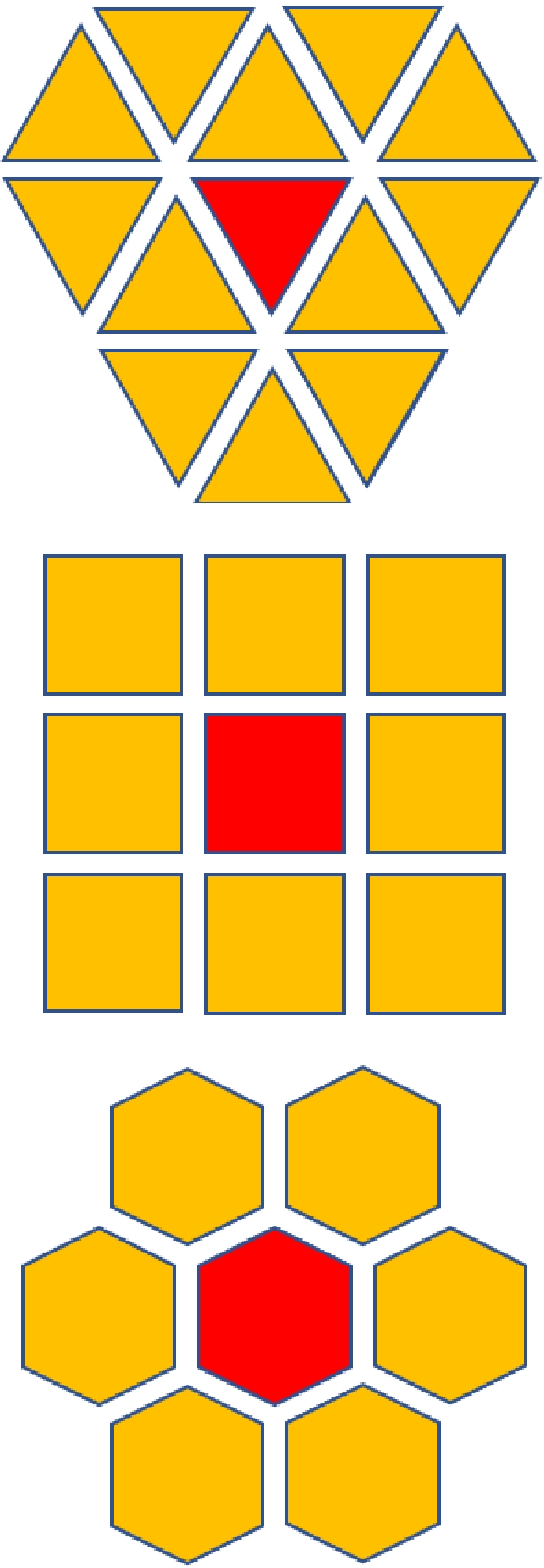
Figure 3.
Triangular, square and hexagonal cellular space.
The prediction model of atmospheric diffusion based on cellular automata is mainly by applying the relevant principles such as fluid dynamics to the evolution rules, using the interaction between cells to dynamically evolve the process of atmospheric diffusion. The flowchart of smoke dispersion prediction using cellular automata is shown in Fig. 4. Wang applied the Gaussian plume model to the cellular automaton and compared the simulation results with other models, showing that using cellular automaton for smoke prediction has better results[71]. Some scholars also use artificial neural networks as the evolution rules of cellular automata[72]. Lauret et al. developed an atmospheric diffusion model combining a two-dimensional planar cellular automaton with an artificial neural network, and the computational speed was 1.5−120 times faster than that of the CFD model[73]. Cao et al. constructed a dynamic prediction model of toxic gas concentration based on the theory of cellular automata, and further constructed a dynamic assessment model of toxic gas leakage accident risk by combining personal risk and social risk, which provides a scientific basis for emergency response decision for toxic gas leakage accidents[65]. Yu & Chang proposed a new method based on three-dimensional cellular automata, using positive hexahedron and von Neumann neighborhood structure as evolution rules, and the model accuracy is comparable to the Lagrangian random particle model, but the operation time is at least 486.4%−564.6% faster than the drift-flux model[74].
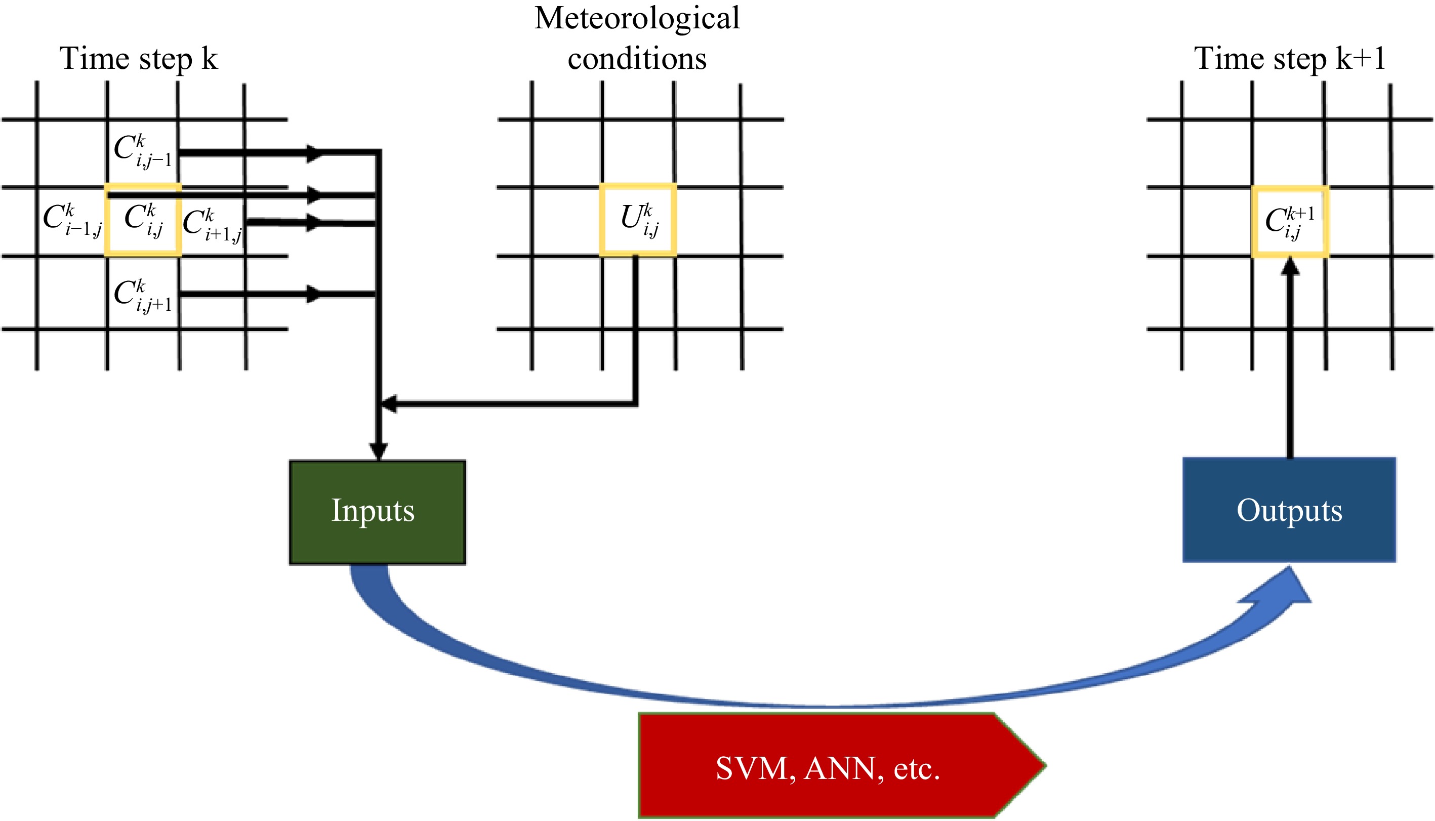
Figure 4.
Cellular automaton state update process.
The atmospheric diffusion process can be simulated through the application of cellular automata by setting the evolution rules between cells rather than complex numerical equations, and in some cases an equivalent accuracy and higher computational speed compared to those of CFD models can be achieved. However, since meta-cellular automata use explicit algorithms and do not have error compensation, they are not suitable for long time predictions. For this issue, the model periodicity can be calibrated using data assimilation techniques and also the evolutionary rules of cellular automata can be developed in depth to further improve model accuracy.
-
With the development of artificial intelligence, historical accident data is fed to artificial intelligence (AI) for model training, which can also achieve good prediction results. According to the different sources of model input, data can be divided into atmospheric dispersion prediction models based on machine learning regression methods and atmospheric dispersion prediction models based on computer vision.
In hazardous chemical atmospheric dispersion accidents, some input parameters needed by empirical and simplified models often cannot be obtained quickly and accurately. Some scholars apply artificial neural networks to atmospheric dispersion prediction, bypassing input parameters such as source information and cloud information that are difficult to obtain or cannot be obtained accurately, and using some easily available data at the scene such as substance concentration, substance properties, meteorological conditions and geographical information as the input to the artificial neural network. Historical accidents are used as the data set to train the artificial neural network for atmospheric dispersion prediction. Some scholars have also applied machine learning models such as SVM[75] to atmospheric dispersion prediction and developed the atmospheric dispersion prediction model based on machine learning regression methods.
Atmospheric dispersion prediction model based on the machine learning regression method
-
Nowadays, machine learning has been widely used in the field of chemical safety, and its main role is to extract the implied patterns from a large amount of historical data and use them for prediction or classification. Artificial neural network is a part of machine learning, which is a complex network consisting of a large number of simple components interconnected with each other, highly nonlinear, capable of complex logic operations and nonlinear relationship implementation, with fast processing speed and strong fault tolerance. Using the powerful computational power of artificial neural networks to fit the complex nonlinear relationship between the accident spread range and the input. When an accident occurs at the site, the trained artificial neural network can be used to quickly predict the spreading range of the leakage material using the accident scene information obtained from sensor acquisition and other monitoring systems. So et al. used a combination of 14 variable values detected by optical sensors, process hazard analysis software tool (PHAST), and artificial neural networks to estimate toxic gas release rates[76]. However, this approach did not predict the future impact on distant areas. Wang et al. combined gas detectors, artificial neural networks, and atmospheric dispersion models to propose a fast prediction method that can predict atmospheric release concentrations using easily available parameters, which can be achieved in remote areas where no source information is available[77]. Jiao et al. built a database including 19 chemicals and 30,022 toxic substances diffusion by using PHAST software to simulate four main parameters of leakage volume, substance quantity, temperature and pressure, and compared three modeling methods, random forest, gradient boosting and deep neural network, and the deep neural network had the highest accuracy with an accuracy variance of 0.994 and root mean square error less than 0.1[78]. Ma et al. designed a series of atmospheric diffusion prediction models based on the machine learning, among which Gaussian-SVM model performed the best, and also incorporated PSO to filter the parameters, and the prediction results were better than Gaussian and Lagrangian random dispersion models[79]. Wang et al. used experimental data from the Prairie Grass project to compare two different machine learning methods in atmospheric dispersion, with different input parameters for the two models. The results show that SVM has better generalization ability in smaller datasets, while back propagation (BP) neural networks may lead to overfitting[80]. Qian et al. proposed an atmospheric dispersion prediction model based on long short term memory (LSTM) with higher accuracy, especially in high concentration dispersion scenarios, in response to the problem that BP neural networks can overfit[81]. Models for atmospheric dispersion prediction using SVM and BP neural networks still need to be improved, and Ni et al. proposed prediction models based on deep confidence networks and convolutional neural networks, and both models were compared with Gaussian models, CFD model, SVM and BP neural network, and the results showed that the model based on deep confidence network and convolutional neural network has the shortest training and prediction time and the highest accuracy, but currently this model is only applicable to certain single point sources of leakage, and to be applicable to more scenarios, the data set of the diffusion model needs to be increased[82]. The machine learning regression-based approach for atmospheric diffusion prediction uses the results of atmospheric diffusion model simulations and the results detected by detectors as inputs to the model for training, which is performed for each scenario, with a large amount of data and some parameters not considered. The atmospheric dispersion prediction based on machine learning regression method uses the results of atmospheric dispersion model simulations and the results detected by detectors as inputs to the model for training, which improves the prediction accuracy and speed, but each scenario has to be trained with a large upfront workload and some parameters are not considered.
Atmospheric dispersion prediction model based on computer vision
-
The data source of the atmospheric prediction model based on the machine learning regression method is obtained by remote transmission, so it also cannot truly restore the accident site information. Computer vision technology extracts useful information from video images to meet people’s requirements, and because of its high real-time and accuracy, its application to the safety field can obtain accurate information about the accident scene. Atmospheric dispersion prediction based on computer vision is achieved by first using unmanned aerial vehicle (UAV) technology, carrying surveillance cameras to obtain real-time site information, and then using smoke recognition models to detect the atmospheric coverage and carry out graphical processing on the basis of recognition to achieve atmospheric dispersion prediction with better accuracy and real-time performance.
Computer vision technology is the use of cameras and computers instead of the human eye to identify, track and measure targets, etc., and further process graphics to obtain images more suitable for human eye observation or transmission to instruments for detection. Until now, many scholars used computer vision technology for online identification and detection of abnormal states of personnel and environment for risk source monitoring and early warning purposes, for example, the identification and detection technology for smoke has reached high accuracy. However, few studies have been conducted to predict the trend of environmental changes based on the identification and detection of environmental abnormal states. Considering the high real-time and accuracy of current computer vision technology and the similarity between smoke and atmospheric dispersion, it could be possible to use this technology to achieve atmospheric dispersion predictions in the future. The current state of smoke recognition research is summarized in this paper, on the basis of which it is pointed out that smoke dispersion in the future time period can be predicted based on the changes of the identified smoke coverage. In addition, considering that gas cloud imaging techniques such as infrared thermography can be used for monitoring chemical gas clouds within non-visible light, the atmospheric dispersion prediction model based on computer vision can be developed based on the formation of a non-visible gas cloud imaging dataset.
The traditional steps of smoke detection algorithms are video acquisition, preprocessing, suspected area segmentation, feature extraction, and classification and identification[83]. The video acquisition phase stage is the process of converting the acquired image information into digital information and transmitting the digital information to the image processing system and computer process through the camera. Common video acquisition tools include visible light cameras[84], infrared cameras, and so on. The preprocessing stage is to expand the dataset and improve the quality of the dataset, and common preprocessing methods are data enhancement, image denoising, etc. The suspected region segmentation stage is to use the salient features of smoke to segment the suspected smoke region, which can reduce the amount and time of operation, and common segmentation methods include data enhancement[85], color segmentation[86], motion segmentation[87], etc. Extracting features unique to smoke can describe the changes in smoke, and by extracting different features can achieve smoke detection. Common smoke features include color[88], texture[89], shape irregularity feature[90], motion direction feature[91], energy analysis[92] and other features. The extracted features are fed to the classifier for training, and after optimal tuning of the parameters, the trained classifier can be used for smoke detection, and common classifiers are support vector machines[93], AdaBoost[94], etc. The complete flow of smoke detection is shown in Fig. 5.
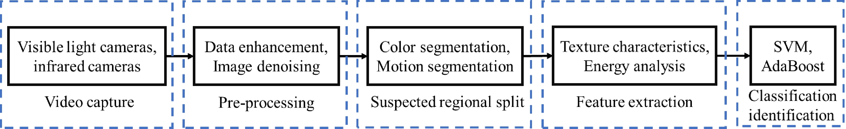
Figure 5.
Flow chart of smoke identification based on computer vision.
The quality of extracted smoke features determines the accuracy of detection, feature extraction often relies on experience, different scenes also need to extract different features, and the generalization ability is not strong. Deep learning can fit complex nonlinear relationships and extract features automatically. Convolutional neural networks play a pivotal role in the study of image recognition, but the accuracy of recognition depends on the quality of the dataset and requires a lot of preliminary preparation work. Applying convolutional neural networks to smoke recognition, a lot of adaptation and optimization work has been carried out by previous authors[95].
Wang et al. extracted motion feature, color feature, background blur, shape irregularity features and main motion direction feature of smoke, used support vector machine to classify, and optimized the parameters using artificial bee colony algorithm[96]. Feng et al. proposed a convolutional neural network based on the target region for fire and smoke recognition, using the background difference method for motion target detection and inputting the extracted motion target regions into the convolutional neural network for classification, with a detection rate of 97.25% and a false detection rate of 6.28%[97]. While Yu et al. were using theoptical flow method to extract the motion features of smoke, the traditional optical flow method is not applicable to the detection of images such as gas and liquids[98]. Wang et al. improved the optical flow field model and proposed the method of using the optimal quality of transmitted optical flow as a low-dimensional descriptor of complex processes, inputting the improved optical flow map and RGB color features into the neural network for feature extraction, and using a supervised Bayesian classifier for judging smoke and flame, which can distinguish between smoke and backgrounds such as white clouds with similar colors[99]. Yang et al. proposed a smoke detection model based on video streams and continuous time domain by combining graph convolutional networks with ordinary differential equations on non-Euclidean structures to extract inter-frame connections[100]. Based on this, Ko et al. combined temporal and spatial information to construct a 3D spatio-temporal body by combining the key frame of smoke with the previous frame to extract the directional optical flow on spatial and temporal features[101]. Ye et al. considered video sequences as multidimensional volume data and proposed a dynamic texture descriptor based on Surfacelet transform and HMT model, and used support vector machines as classifiers. The Surfacelet transform decomposes the high-frequency signal into different scales and directions. The improved model provides an approximation of the coefficients of the Surfacelet transform using the 3D HMT model, and describes the texture features using the joint probability density of the coefficients, which has higher accuracy than the local binary pattern and the grayscale coeval matrix[102]. Yuan et al. reduced the false alarm rate by segmenting video images into equal-sized blocks and studying the accumulation on the main motion direction and duration motion time of each block on the video sequence[103]. Kim et al. extracted suspected smoke regions by the Gaussian mixture model and detected smoke in candidate regions using Adaboost[104]. For small smoke, Yuan et al. proposed a dual-threshold AdaBoost and the step search technique combined with image smoke detection methods based on Haar features to improve the generalization ability[105]. Chen et al. then proposed a backbone feature extraction network combining enhanced attention mechanism module, residual module, and SPP module to fuse multi-level feature map vectors and cover multi-scale target features, which improved the detection accuracy of small targets and reduces the convolution parameters[106]. For the problem of blurred smoke images and complex and variable backgrounds, Yuan et al. proposed an end-to-end SInception network based on GoogLeNet Inception v3 and SE Block, and established bimodal feature fusion of dark channel images for this network, using image enhancement techniques and generating adversarial networks to expand the data. On the enhanced dataset, the accuracy was improved to 99.65 % and the speed was reduced to 0.26 milliseconds[107]. Lin proposed a two-way 3D convolutional neural network to extract temporal features for smoke detection[108]. Yang proposed a smoke video detection system, which detected smoke hierarchically by the 2D lightweight MobilenetV2-SSD smoke detection algorithm and the 3D-RD Net smoke dynamic detection algorithm. Figure 6 shows smoke detection using the recognition model[109].
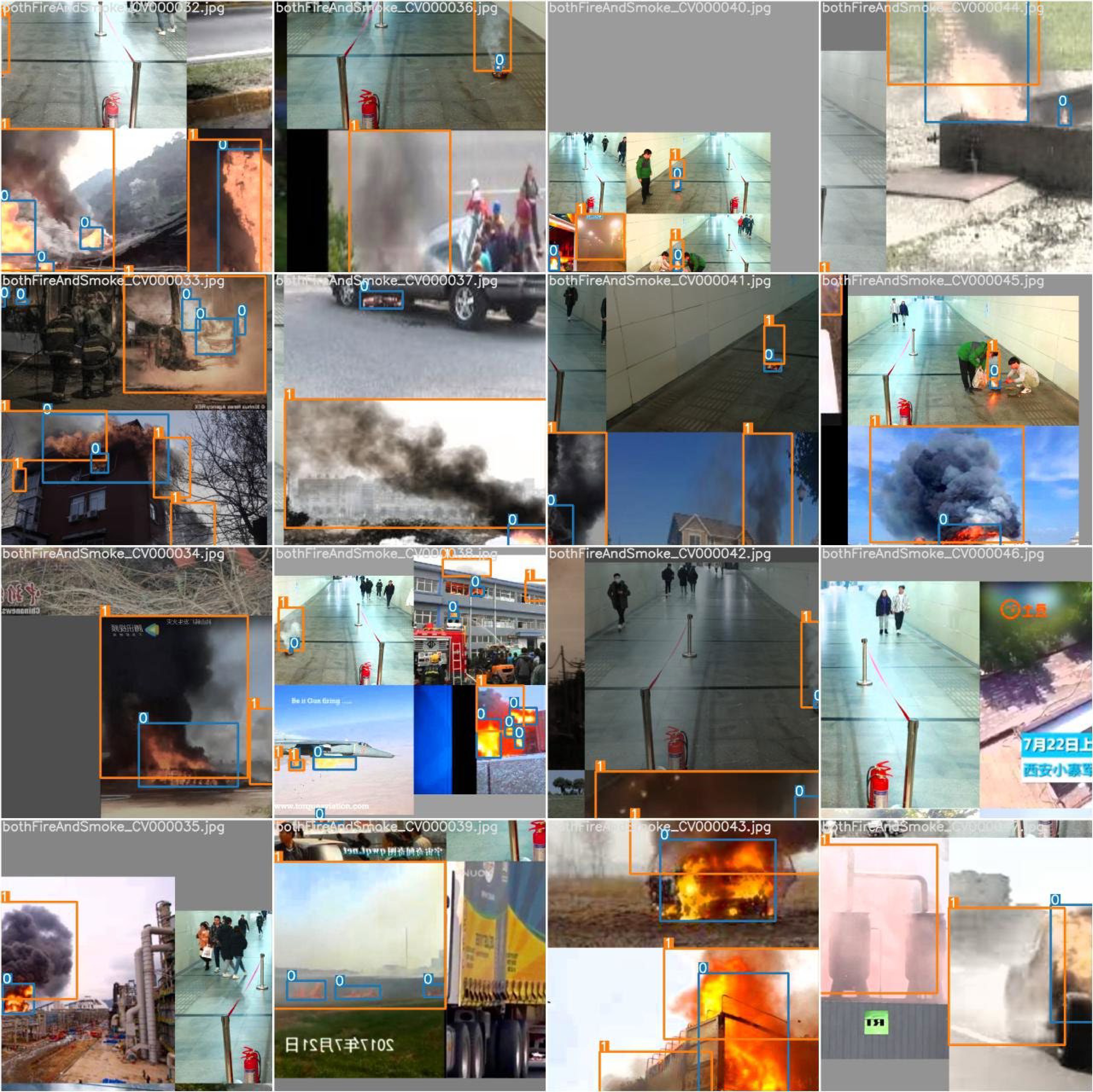
Figure 6.
Smoke recognition using computer vision.
At present, smoke recognition research has developed to a very mature point, and the accuracy of recognition can meet the emergency requirements, but none of the related scholars have continued the research on atmospheric dispersion range prediction and traceability. Atmospheric dispersion prediction based on computer vision is still in the theoretical stage, and the complexity of the atmospheric dispersion process also puts high demands on the model, but the integration of other cutting-edge technologies, such as image processing technology and drone technology, and the application of real-time and accuracy of computer vision to smoke dispersion prediction can improve the existing level of emergency response to hazardous chemical accidents. Chang et al. connect cameras to devices such as drones and transmit the acquired accident scene video to a cloud server to send to a trained target detection model. Incident commanders decide the number of fire trucks and firefighters and other scene conditions based on the model detection results, and the fatigue and survival status of firefighters are also determined, so that once a firefighter is found to be unwell, incident commanders can immediately implement rescue[110].
-
Simplified-experience models and mechanism- and rule-driven models for atmospheric dispersion prediction are well established, and some organizations have developed many applicable professional applications based on these two types of models, including PHAST, ALOHA, FLACS, PyroSim, etc., which can provide guidance suggestions for emergency decision-making. Meanwhile, the accident dispersion information database is one of the factors affecting the accuracy of the mechanism- and rule-driven models[111], and a large database of accident information can be simulated using professional application software. Jiao et al. used PHAST to build a database including 30,022 toxic substances dispersion[78], I et al. used FLACS simulation results for quantitative analysis[112]. Four main professional applications are described below, where PHAST and ALOHA use simplified-experience models, FLACS and PyroSim use the mechanism- and rule-driven models, and research for the third type of atmospheric dispersion prediction models is still incomplete, and there are no mature professional applications.
PHAST
-
PHAST (Process Hazard Analysis Software Tool) is developed independently by Det Norske Veritas for hazard analysis and safety calculations in oil, is a software for hazard analysis and safety calculations in the oil, petrochemical and gas sectors[113]. PHAST uses the UDM model as the leakage dispersion module to count the concentration distribution at the same moments of the interval, connect them into concentration lines, describe the width of the cloud and the downwind distance, and derive the safe area, flammable and explosive area, and quasi-hazardous area. The UDM module simulate the concentration dispersion of atmosphere pressure, high pressure, unidirectional and two-phase leakage, and is divided into five modules: diffusion of jet streams; droplet evaporation and condensation, cloud landing process; liquid pool expansion and evaporation; heavy gas diffusion; and passive diffusion. Gerbec et al. & Witlox et al. studied heavy atmospheric diffusion using the UDM module with good predictions[114,115], and Pandya et al. investigated the importance of parameters during the diffusion of nitric oxide, ammonia and chlorine leakage using PHAST[116]. PHAST is suitable for leakage diffusion prediction of transient, continuous, neutral gas, and heavy gas leakage by entering the type of equipment, type of substance, storage parameters, leakage mode, surrounding environment (atmospheric temperature, humidity, stability, wind speed) and other settings, and output the scope and extent of the impact of possible fire and explosion accidents, which can be used to assess the rate of substance leakage, consequences of fire, consequences of explosion, and consequences of toxic atmospheric leakage[117]. The main function of PHAST is to simulate and predict the dangerous consequences of safety accidents generated by oil and gas through mathematical models, including toxic gas leakage, flash fire, jet fire, pool fire, fireball, explosion, etc., and the UMD module can simulate the complete accident scenario process from initial leakage to termination.
ALOHA
-
Areal Locations of Hazardous Atmospheres (ALOHA) is developed by the Emergency Response Division (ERD) of the National Oceanic and Atmospheric Administration (NOAA) in cooperation with the office of emergency management of the Environmental Protection Agency (EPA). Its primary purpose is to provide emergency responders with area-wide assessments of some of the common hazards associated with chemical leakage. ALOHA provides simulations of the extent of some of the hazardous areas associated with short-term accidental leakage of volatile and flammable chemicals, while also addressing the personal risks associated with toxic chemical vapor inhalation, thermal radiation from chemical fires, and blast waves from vapor cloud explosions. ALOHA contains a large database of chemical properties and geographic information containing data on the physicochemical properties and toxicity of approximately 1,000 common hazardous chemicals. The mathematical models in ALOHA include Gaussian models for neutral gas and some models for heavy gas that can predict dispersion areas ranging from about 100 m to 10 km, with durations up to one hour, for wind speeds greater than one meter per second (at 10 m), and should not be used in very low or calm wind conditions.
FLACS
-
FLACS is a 3D computational fluid dynamics software developed by Gexcon Norway, which is the world's leading fire and explosion risk assessment software and is widely used in the oil and gas, chemical, and nuclear power industries. FLACS software is widely recognized by many international standards such as 49 CFR 193.2059 of US Federal Regulation and NORSOK Z-013 of Norwegian Petroleum Technical Regulation and Standard, and is the only CFD software currently approved in the U.S. for the simulation of all LNG vapor dispersion scenarios required in the siting of onshore LNG facilities, with reliable simulation results.
FLACS includes CASD (set the scene module), FLOWVIS (results processing module), GasEx (explosion module), Dispersion (diffusion module), Hydrogen (hydrogen module), DustEx (dust module), Fire (fire module), Blast (solid explosion module) and Risk (risk module). Many scholars at home and abroad use this software for numerical simulation studies of hydrogen leakage, diffusion and explosion. Holborn et al. used FLACS to simulate the downwind hazard distance and liquid pool size for LH2 leakage dispersion and the combustible mass of hydrogen clouds under different environmental conditions and release scenarios[118]. Hansen verified that FLACS can be used to simulate the smoke dispersion of LNG leakage accidents[119].
-
Hazardous chemical accidents are sudden and hazardous, causing great damage to people’s lives and properties, and good accident prediction is of great significance to natural ecology and social stability. It is the future development trend to solve the drawbacks of traditional atmospheric diffusion prediction models, improve the automation level of monitoring, enhance the real-time, robustness and accuracy of atmospheric diffusion prediction, and use intelligent tools to monitor leakage and make diffusion prediction directly. With the development of computer vision, its application to the safety field can solve some limitations of existing models. The data sources of computer vision are easily accessible, which can be obtained directly through UAV photography, and the smoke can be identified and predicted by recognition algorithms, which can meet the real-time requirements, and the trained models can be applied to different scenarios. The future development trend of atmospheric dispersion prediction models is summarized in this paper, as shown in Fig. 7.

Figure 7.
Future research directions
Future research directions
Development of an emergency response system based on full-scene atmospheric dispersion simulation
-
Although the simulation speed of Simplified-experience models is fast, they are mostly suitable for atmospheric diffusion in flat areas, while the mechanism- and rule-driven models can be applied to complex terrain, but it is complex and time-consuming to calculate and is not suitable for use in an emergency. Optimize the existing models, combine GIS technology and data fusion and other technologies, analyze the accident site conditions comprehensively, select different diffusion models independently for dynamic simulation according to different conditions, and develop an atmospheric diffusion prediction emergency system that can adapt to the whole scenario.
Integrate image processing technology
-
Using unmanned aerial vehicle technology to obtain accident video data in real time, extract features from the image, then classify the image according to the geometric and texture features of the graphic, and analyze the structure of the entire image. The material monitored by computer vision technology is geometrically corrected, and image processing technology is used to show the leakage and diffusion range in the future in the video image directly, which can realize real-time prediction of the leakage range and has good robustness.
Establish a database of historical accident scenario information and meteorological information
-
Ninety-nine percent of the CFD simulation time is used for wind field calculation, and a rich wind field information database could be established in advance, which can greatly save simulation time. The database could be established by counting the wind field information of specific sites or by using CFD model simulations, which should include leakage scene information (such as leakage substance, leakage source location, leakage rate and leakage volume, etc.) and meteorological information (such as wind speed, wind direction, temperature, pressure, etc.). Model a specific site in advance, simulate the flow field calculation, and use the difference calculation to reduce the error caused by the large difference between the scene and the database. Combine with optimization algorithms to study more accurate difference estimation methods and improve the database generalization capability.
Study of new correction algorithms
-
To determine the appropriate evolution rules for various phenomena during gas diffusion, Gaussian models, SVMs and artificial neural networks have been applied as evolution rules for cellular automata by previous authors, and the simulation can achieve good real-time performance. However, even if the performance of SVM and artificial neural networks are well trained, with the increase of time step, errors will be accumulated and cause large differences to the final simulation results. It is important to investigate new correction algorithms to eliminate the accumulation of errors, calibrate the model parameters, reduce the differences between predicted and real values, and better simulate the diffusion process of the atmosphere.
-
The atmospheric dispersion of hazardous substances is a complex fluid motion process governed by various factors such as atmospheric environment, geographic topography and chemical reactions of substances. Until now, numerous researchers have conducted a large range of experiments and established many gas leakage dispersion models, such as phenomenological model, box and similar model, shallow model and 3D hydrodynamic model, etc., and accordingly developed various atmospheric dispersion prediction software. Based on the previous literature summary, in this paper, the current atmospheric dispersion prediction models are classified into three categories according to the theoretical approach of model construction: (1) Empirical model developed through the simplification of atmospheric dispersion apparent phenomenon; (2) Prediction model derived from the physical-chemical mechanisms and laws of atmospheric dispersion; (3) Data-driven atmospheric dispersion prediction model.
Most empirical models are developed through simplifying the information of actual accident scenes with mathematical expressions. In general, these models are of simple structure and fast calculation speed, and so they have been most widely employed around the world. However, the prediction time and range of such models are small. For instance, the obtained parameters are always of great uncertainty, the prediction accuracy is generally lower with large error in complex scenarios.
Prediction models derived from the physical-chemical mechanisms and laws of atmospheric dispersion transfer the physicochemical laws of atmospheric dispersion to computers for simulation, which have the advantages of controllable boundary conditions, user-defined fluid parameters, applicability to complex terrain conditions, and good computational repeatability. It can completely describe the atmospheric diffusion phenomenon with better applicability and accuracy. However, like the empirical models, these kinds of models also make various assumptions and simplifications for the accident scene, so it cannot fully simulate the actual environment. Moreover, it is computationally intensive and time-consuming, making it unsuitable for industrial emergency scenarios.
Unlike the non-data-driven atmospheric dispersion prediction model that makes more simplifications and assumptions about the accident scene information, which leads to great differences between the model prediction results and the actual situation, the data-driven models apply artificial intelligence to atmospheric diffusion prediction, which have a few assumption of scene information with fast operation speed, so this kind of model has a good development prospect. This kind of model uses two methods, one is machine learning, the other is computer vision. Wang's research[77] shows that the machine learning method can accurately predict the diffusion of substances in the atmosphere when the source of substance release is unknown. But the prediction model has a large workload in the early stage, can only be calculated in two-dimensional space and the influence of obstacles and boundaries is not considered in the modeling process, so it has some limitations. The computer vision method uses accident video images as input information, which can hopefully achieve real-time restoration of the accident site. In this regard, the research status of this kind of model is discussed in detail in this paper, finding that there are few relevant studies. Most of the research work only involves the identification of released substances, and few scholars carry out the research of atmospheric diffusion prediction based on substance identification.
In summary, traditional empirical models and mechanistic models still have various problems in terms of accuracy, computational efficiency and model applicability, while the data-driven models are still immature. In the future, it is still necessary to deepen the above three types of models, especially in combination with cutting-edge technologies such as artificial intelligence, unmanned aerial vehicles and geographic information systems, to further promote the development of atmospheric diffusion prediction research.
We gratefully acknowledge the financial support provided by the Fundamental Research Funds for Central Universities (BUCTRC202014).
-
The authors declare that they have no conflict of interest.
- Copyright: © 2022 by the author(s). Published by Maximum Academic Press on behalf of Nanjing Tech University. This article is an open access article distributed under Creative Commons Attribution License (CC BY 4.0), visit https://creativecommons.org/licenses/by/4.0/.
-
About this article
Cite this article
Dou Z, Liu Z, Li L, Zhou H, Wang Q, et al. 2022. Atmospheric dispersion prediction of accidental release: A review. Emergency Management Science and Technology 2:9 doi: 10.48130/EMST-2022-0009 

Atmospheric dispersion prediction of accidental release: A review
- Received: 22 June 2022
- Accepted: 08 August 2022
- Published online: 31 August 2022
Abstract: Modern industrial development is accompanied by the increasingly frequent occurrence of accidental release atmospheric dispersion events, causing extremely serious human and property losses and environmental pollution, in which rapid and accurate prediction of atmospheric dispersion is an important task to mitigate the unexpected consequences. In this paper, we take the case of previous years as the starting point, firstly, the occurred hazardous chemical atmospheric dispersion accidents in the past five years are shown, and the related concepts of hazardous chemical atmospheric dispersion are given. Then, the current state of atmospheric dispersion research is reviewed, well-known experiments on atmospheric dispersion of hazardous chemicals are summarized, and correspondingly the existing atmospheric dispersion prediction models are classified into simplified-experience models, mechanism- and rule-driven models and data-driven models. In particular, for the purpose of rapid atmospheric dispersion prediction, some research on atmospheric detection and identification are analyzed in detail. Moreover, the relevant professional software for atmospheric dispersion prediction are introduced, and also their calculation adaptabilities regarding time-consumption and output accuracy are discussed. Thereinafter, according to the shortcomings of existing atmospheric dispersion prediction models in research and application fields, the development trend of atmospheric dispersion prediction research and technology is foreseen, and some feasible future research directions are proposed as follows: (1) the fusion of image processing techniques, the establishment of a database of historical accident scene information and meteorological information, (2) new correction algorithms, and (3) an emergency response system for full-scene atmospheric dispersion prediction.
-
Key words:
- Atmospheric dispersion prediction /
- Accidental release /
- Models' review /
- Hazardous chemicals /
- CFD /
- ANN