


-
Plant water status is widely recognized as an important factor in attaining a high-quality grape due to its role in vegetative growth, partitioning mechanism, berry development, and metabolic composition[1−4]. However, grapevine water status (GWS) exhibits spatial variability across vineyards under a homogeneous irrigation regime, leading to variation in berry development and quality[5,6]. Management of the spatial variability of GWS across vineyards can potentially benefit growers due to berry quality optimization[7,8]. To help achieve optimization of quality, provision of spatial (across vineyards) and temporal (along growing season) GWS monitoring maps would be very useful to the vineyard managers.
Electromagnetic reflectance obtained from remote sensing (RS) platforms, such as satellites and uncrewed aerial vehicles (UAVs), has gained popularity for acting as proxies for GWS. RS techniques enable spatial monitoring of GWS within vineyards, so its application can be applied to develop site-specific irrigation or assist in decision-making for irrigation management. Compared to satellites, UAVs mounted with sensors have the relative advantages of flexibility in flight scheduling, imagery with a higher spatial resolution (at centimeter-scale), and lower cost of operation. However, UAV surveys are confined to smaller areas due to the short flight endurance imposed by their payload[9]. This may lead to the introduction of non-negligible uncertainty in the radiometric quality of orthoimages resulting from mosaicking a large number of tiles[10]. Satellites, compared to UAVs, are superior when mapping at a larger scale within a single acquisition on a regular basis, guaranteeing radiometric homogeneity for all pixels in the scene[10]. Nevertheless, when considering crops with discontinuous layouts, such as vineyards, satellite imagery with low to moderate resolution cannot be reliably used for plant status description due to the biased assessment originating from the presence of inter-row vegetation and bare soil[11,12]. Although there are some satellites (e.g. GEOSAT-2, GeoEye-1, WorldView-3) that offer images with high resolution and can be used for field monitoring in viticulture, the cost of image acquisition makes it impractical in the application of irrigation scheduling that needs regular monitoring. The challenge when using RS tools for timely monitoring of highly dynamic phenomena, such as GWS monitoring, is to obtain data that not only has high spatial and temporal resolution but also is affordable and timely accessible.
Pla et al.[13] used UAV data as reference to calibrate Sentinel-2 imagery to quantify damage in rice crops. This study demonstrated that the calibration approach can serve as a viable and cost-efficient alternative to retrieve biophysical variables on large scales. Revill et al.[14] later developed a two-stage method for the calibration of satellite vegetation indices (VIs) to approximate crop leaf area index by calibrating UAV images with ground measurements, followed by calibrating satellite images with calibrated UAV data. This new methodological framework provides an opportunity to integrate the advantages of both satellites and UAVs by utilizing UAV data to help bridge ground truthing and satellite images. This will enable variables of interest to be retrieved at a larger scale, while removing the spectral response of the inter-row elements during the calibration process. This will enhance the reliability of the use of satellite data for plant status monitoring. Based on the study of Revill et al.[14], Bukowiecki et al.[15] transferred this approach to green area index estimation based on the data collected over four growing seasons. The satellite-based prediction model achieved a high performance (coefficient of determination of 0.82). Mazzia et al.[16] used a convolutional neural network to refine satellite-based normalized difference vegetation index maps by utilizing UAV-derived information. They found the refined maps could better describe crop status in terms of correlation analysis and ANOVA, in comparison to the raw satellite images. However, the delivery of satellite imagery to the end user is not in real-time after the fields are sensed. There are often delays in data transfer to the ground station, handling, and distribution to the user, while some processes (such as geometric, radiometric, and atmospheric corrections) are needed before image analysis[17]. In addition, the application of satellite imagery over open fields is weather-dependent and illumination sensitive. Cloud and fog interference is a common restriction imposed on the usability of satellite-based data for crop monitoring. This requires the user to wait for the next revisit of data acquisition[18,19]. These constraints are likely to compromise the practicability of the satellite imagery for growers and viticulturists, despite the satellite images being calibrated with ground truthing. Thus, there is a clear requirement to develop tools for GWS forecasting to promote precision irrigation and thus berry quality.
To potentially address the inaccessibility of satellite-based data caused by unfavorable weather, one way is to develop a GWS prediction model using a soil water balance. As GWS is an integrative response to soil moisture availability, water usage by plants, evaporation, atmospheric transfer, and canopy structures[20], there is potential to simulate the changes in GWS along a growing season by using these variables as predictors. Precipitation, irrigation, and fertigation replenish soil water content, thus positively impacting GWS[21]. Evapotranspiration (quantifying the net loss of water vapor from evaporation and plant transpiration) accounts for the dynamics and interrelationships of weather components, vegetation expression, and soil properties[22]. Soil properties and topography have persistent effects on the spatial distribution of soil water, which determines the soil moisture availability to plants, and thus may influence GWS[23]. Cultivation management, such as leaf plucking and trimming, alters canopy vigor, shoot distribution, and total leaf area, leading to the regulation of water consumption level by grapevines[24]. Seasonality, noted as day of the year (DOY), has been found to explain a large part of the variability in GWS[25].
Machine learning (ML) models have recently been extensively used in RS applications due to their ability in modeling both linear and non-linear relationships[26]. These models can be applied to multi-dimensional problems, so they can potentially simulate spectral, spatial, and temporal variabilities between images from different platforms, as well as the complex relationships between GWS and predictors. Previous studies have shown the potential of using UAV or satellite-derived VIs to assess GWS[12,23,27−32]. However, these assessments were mostly limited to identifying the relationships between UAV-based or satellite-based data, and GWS, without considering the need for real-time monitoring which is constrained by the time required for post-processing and associated weather-dependent issues. Most of the RS platforms are currently not able to provide real-time information which is especially important in the context of dynamic GWS monitoring. This study aims to provide GWS prediction based on two-stage calibrated satellite images, which caps off the two previous studies[33,34] with a prediction tool to assist growers and viticulturists in irrigation scheduling or related management decisions for vineyards. Wei et al.[33] focused on identifying the most related spectral features with changes in GWS, and it turned out that they dispersed across multiple spectral bands and needed to be computed collectively using multivariate models. Wei et al.[34] highlighted the importance of ancillary variables (vegetation data, temporal trends, weather parameters, and soil/terrain characteristics) in helping a multispectral sensor describe the variation of GWS. The procedures of this study undertaken were (i) using two-stage calibration (based on ML models) to acquire calibrated satellite images exhibiting GWS estimations for a series of acquisition dates across the first growing season. (ii) developing a GWS prediction model by regressing against the calibrated satellite images acquired in the first growing season using ML models. (iii) evaluating this prediction model by validation with a second set of ground measurements independently collected in the second growing season. To the authors' knowledge, this is the first study that a two-stage calibration approach has been employed to calibrate satellite images for developing GWS prediction models based on ancillary information collected in the first growing season, along with independent evaluation with data collected the second growing season.
-
The study vineyards are located at Martinborough in the Greater Wellington Region (lower North Island) in New Zealand (NZ). Both vineyards are sited on a complex of recent alluvial soils overlying gravels, located close to the Ruamahanga and Huangarua Rivers (Fig. 1). The study site contains two commercial vineyards owned by Palliser Estate, named Wharekauhau and Pencarrow. Our study areas in these two vineyards are 6.6 and 6.7 ha, respectively. Pinot Noir was chosen as the target variety in this study, due to its requirement for relatively precise GWS management. The Pinot Noir vines in both vineyards were planted in the vineyards in 1998−2000 and two-cane vertical shoot positioned. Inter- and intra-row planting space is 2.2 × 1.6 m for Wharekauhau and 2.2 × 1.8 m for Pencarrow. The annual growth cycle of grapevine in NZ comprises budburst, shoot growth, and flowering (September–November), fruit set and veraison (December–February), followed by berry development and harvesting (March–May). From flowering to veraison, the management of GWS critically determines the final berry quality[35,36]. The study periods span 15th November 2020 to 2nd February 2021 for the first growing season (2020/2021) and 23rd November 2021 to 21st January 2022 for the second growing season (2021/2022). This study focused on cultivation practices, including irrigation, fertigation, plucking, and trimming, due to their potential effects on GWS. Both vineyards are drip-irrigated, with the distance between drippers being 0.6 m. The drip rate is 1.2 L/h for the drippers in Wharekauhau, and 1.3 L/h for the drippers in Pencarrow. The irrigation events took place for 2.5 h on each irrigation date. Fertigation was applied to provide additional nutrients, and lasted for 6 h on each date of fertigation. Leaf plucking was implemented to remove 80% of the leaves at one side of the canopy to allow sprays better access to grapevines. Trimming was carried out on top of, and on both sides of, canopies to control vegetative growth. Weather information and cultivation practice events are displayed in Fig. 2.
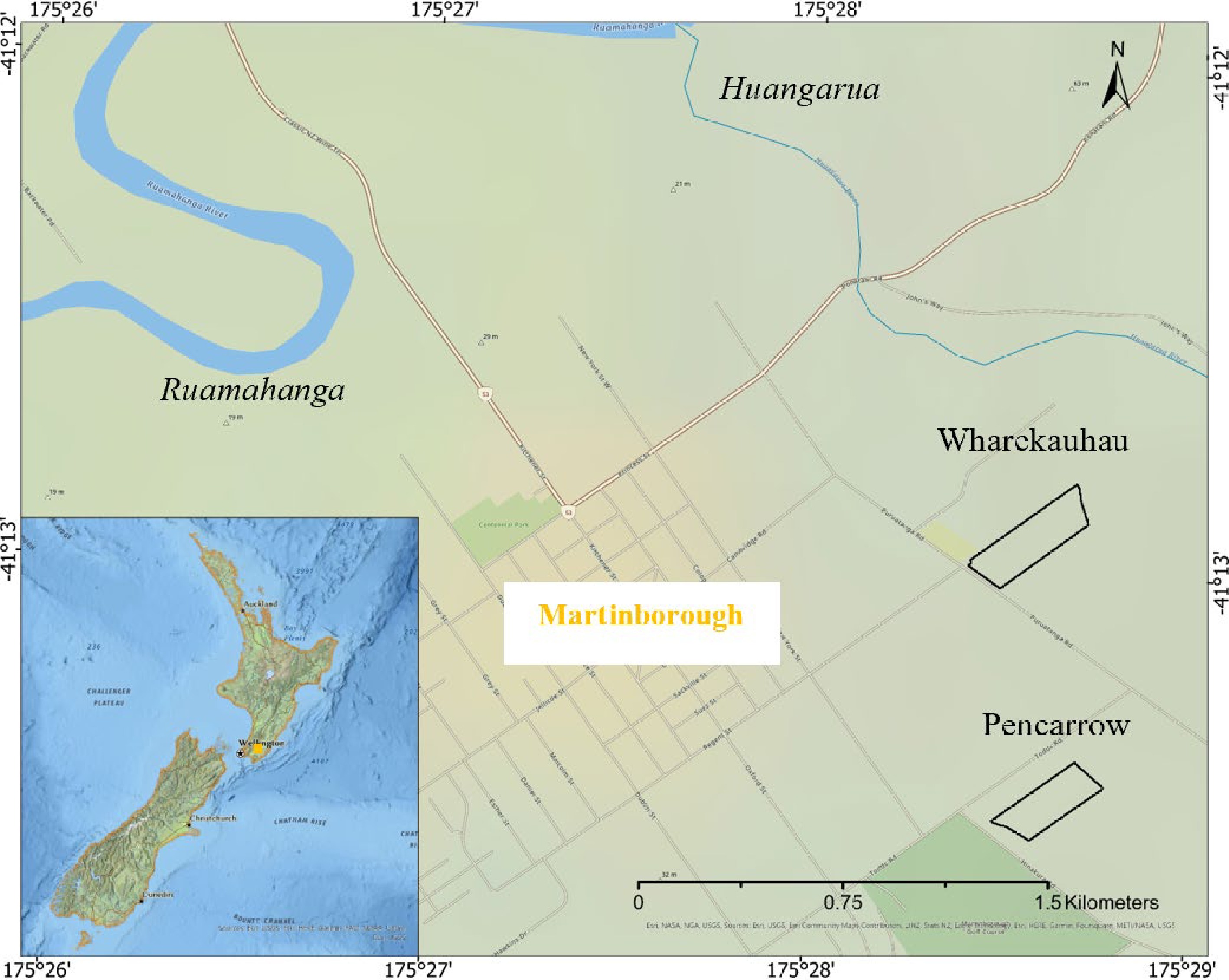
Figure 1.
Location of study vineyards (Source: Esri, USGS).
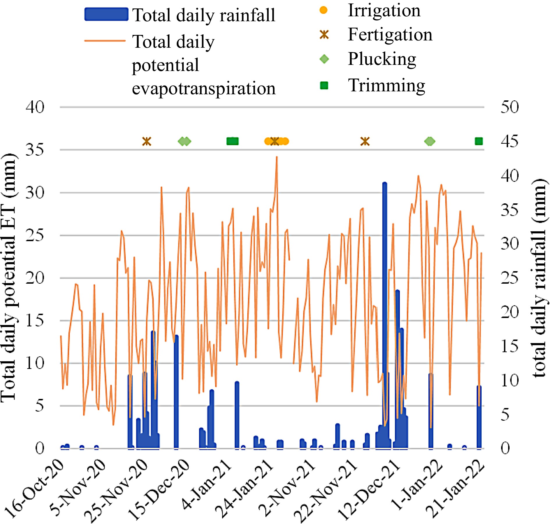
Figure 2.
Total daily potential evapotranspiration and total daily rainfall provided by an on-site weather station, with cultivation practices implemented during the two growing seasons.
Measured data
-
Stem water potential (Ѱstem) was chosen as an indicator for GWS because it has been reported as a comprehensive expression for early water deficit in vines during the day[37]. Several healthy vines were sampled in grids to assess variability across the vineyards for each measurement date (Table 1) using two mature and fully expanded leaves from the middle part of each sampled canopy. These leaves are more representative of the canopies. A pressure chamber (model: 610, MPS, Albany, NY, USA) was used between 13:00 and 15:30 to acquire Ψstem (kPa). Prior to the measurement, the sampled leaves were covered with sealable plastic bags for approximately 1 h. The mean value of the two leaf measurements per vine represents the canopy Ψstem. A total of 85 and 63 separate canopies were sampled in the first and the second growing season, respectively. Each of their trunk locations was recorded using a global navigation satellite system (GNSS) with real-time kinematic (RTK) correction (model: GPS1200+, Leica Geosystems AG., Heerbrugg, Switzerland).
Table 1. Details of data acquisition for measured Ψstem, DJI Phantom 4 multispectral UAV imagery, and PlanetScope satellite imagery. The orange letterings indicate the UAV-satellite image pairs used in the second calibration. UAV = uncrewed aerial vehicle.
Acquisition date Data source Time gap (d) 15/11/2020 Satellite − 16/11/2020 Satellite − 27/11/2020 Measured/UAV − 02/12/2020 Satellite − 04/12/2020 Measured/UAV 1 05/12/2020 Satellite 15/12/2020 Satellite − 17/12/2020 Satellite − 31/12/2020 Satellite − 04/01/2021 Satellite − 14/01/2021 Measured/UAV/
Satellite0 15/01/2021 Satellite − 22/01/2021 Measured/UAV 1 23/01/2021 Satellite 26/01/2021 Satellite − 01/02/2021 Measured/UAV 1 02/02/2021 Satellite 23/11/2021 UAV − 29/11/2021 Measured/UAV − 09/12/2021 Measured/UAV − 11/01/2022 Measured/UAV − 21/01/2022 Measured/UAV − UAV-based data
-
UAV images were collected between 11:00 and 13:00 under cloudless conditions to minimize the impacts of sun angle and shadow. UAV flights and Ѱstem measurements were operated on the same dates to ensure comparability (Table 1). The reflectance, with a spatial resolution of 0.05 m, was recorded by a DJI Phantom 4 multispectral UAV (DJI, Shenzhen, China) with six built-in sensors, including blue (450 ± 16 nm), green (560 ± 16 nm), red (650 ± 16 nm), red edge (730 ± 16 nm), and near-infrared (840 ± 26 nm) regions. An integrated sunlight sensor on the top of the UAV records irradiance in the same bands captured by the multispectral sensor during the flight. This information enables UAV images to be normalized and allows for comparison between images taken under different illumination conditions. Pix4Dmapper (Pix4D SA, Lausanne, Switzerland) was used to apply photogrammetric processing to the UAV data to generate digital surface models (DSM), digital terrain models (DTM), and reflectance maps. To increase imagery spatial accuracy, several ground control points were obtained by GNSS-RTK for each vineyard, and post-imagery alignment was performed in ArcGIS Pro 2.9 (ESRI, Redlands, California, USA).
The vineyards are characterized by discontinuous vegetation surfaces, requiring separation of canopy pixels from grass and soil pixels to obtain pure information of grapevines. As there is a height difference between grapevines and their surrounding components, canopy height can be acquired by subtracting DTM from DSM, then creating binary imagery to exclude background pixels. There are 16 vegetation indices, chosen according to the frequency of usage in viticulture[38], shown in Table 2 and calculated based on pure canopy pixels using 'zonal statistic as table' in ArcGIS Pro.
Table 2. List of vegetation indices used in this study.
Vegetation index Formula Reference Red Edge Chlorophyll Index (NIR/Red edge) − 1 [39] Difference Vegetation Index NIR − Red [40] Enhanced Vegetation Index 2.5 × (NIR − Red)/(NIR + 6 * Red − 7.5 × Blue + 1) [41] Excess Green Index 2 × Green − Red − Blue [42] Green Normalized Difference
Vegetation Index(NIR − Green)/(NIR + Green) [43] Modified Chlorophyll Absorption Ratio Index ((Red edge − Red) − 0.2 × (Red edge − Green)) ×
(Red edge/Red)[44] Modified Soil Adjusted
Vegetation Index(2 × NIR+1 − ((2 × NIR + 1)2 − 8 × (NIR − Red))1/2)/2 [45] Modified Triangular
Vegetation Index1.2 × (1.2 × (NIR − Green) − 2.5 × (Red − Green)) [46] Normalized Difference
Red Edge Index(NIR − Red edge)/(NIR + Red edge) [47] Normalized Difference
Vegetation Index(NIR − Red)/(NIR + Red) [48] Normalized Difference
Green/Red Index(Green − Red)/(Green + Red) [40] Optimized Soil Adjusted
Vegetation Index(NIR − RED)/(NIR + Red + 0.16) [49] Red: Green Ratio Red/Green [50] Simple Ratio NIR/Red [51] Transformed Chlorophyll
Absorption Reflectance Index3 × ((Red edge − Red) − 0.2 × (Red edge − Green) ×
(Red edge/Red))[52] Visible Atmospherically
Resistant Index(Green − Red)/(Green + Red − Blue) [53] Satellite-based data
-
PlanetScope (PS) imagery was chosen for this study mainly due to its high spatial and temporal resolution. PS Constellation, owned by Planet, is composed of approximately 200 'Dove' microsatellites, operating in sun-synchronous orbits and able to provide daily land surface imagery at nadir for the entire Earth, passing the equator between 9:30−11:30 (local solar time)[54]. The product used in this study is PS Analytic Ortho Scene Surface Reflectance, which consists of level 3B images recorded by instrument PSB.SD in coastal blue (431−452 nm), blue (465−515 nm), green I (513−549 nm), green II (547−583 nm), yellow (600−620 nm), red (650−680 nm), red edge (697−713 nm), and near-infrared (845−885 nm) bands. These images are acquired with a ground sample distance of 3.7−4.1 m and then resampled to 3.0 m for distribution. This product is orthorectified to remove geometric distortions, and its positional accuracy is less than 10 m RMSE at the 90th percentile. Radiometric corrections are applied to convert pixel values to at-sensor radiance, while atmospheric corrections are implemented to acquire surface reflectance values. Although PS imagery is superior in terms of spatiotemporal resolution, there is radiometric inconsistency due to cross-satellite differences in spectral response, radiometric quality, and orbital configuration[55,56]. This heterogeneity was addressed in this study by incorporating the radiometric variability in the modeling processes. PS images, covering the study vineyards and obtained on 13 different days over the study period in 2020/2021, were selected for further analysis after cloud and cloud shadow screening (Table 1).
Soil and terrain data
-
An EM38-MK2 is an electromagnetic induction (EMI)-based sensor (Geonics Ltd., Mississauga, Ontario, Canada). The return reading, apparent soil electrical conductivity (ECa), is considered a function of soil texture, soil solution, and soil water content[57]. ECa was used as a proxy to estimate the spatial variation of GWS[58]. In this study, the EM38-MK2 was operated in the vertical dipole mode, with the instrument taking integrated ECa measurements at about 1.5 m depth. An EMI survey was undertaken by towing the EM38-MK2 at the back of an all-terrain vehicle, with a Trimble Yuma tablet (including an onboard GPS receiver) to geo-reference all ECa points (mS/m). The vineyards’ subsurface infrastructure was confirmed with the vineyard manager to ensure there was no interference from buried metal objects. ECa points were measured approximately every 3−10 m along transects that were 10 m apart. Point values less than 0 mS/m were removed before interpolation. The geostatistical interpolation method, Empirical Bayesian Kriging, was used to convert point data into a raster with 1 m resolution.
Elevation (m) for the vineyards was obtained from the 'Wellington LiDAR 1m DEM (2013−2014)' layer provided by Land Information New Zealand data service (
https://data.linz.govt.nz ). This digital elevation model (in 1 m resolution) was created by aerial LiDAR for the Greater Wellington region (captured between 2013 and 2014). Slope (degree) information was derived based on elevation.Meteorological and temporal data
-
Weather data was recorded by the on-site weather station (175.4741, −41.2247 WGS84) established by HARVEST.com (
http://harvest.com ). The variables captured include rainfall (mm) and potential evapotranspiration (PET; mm). Rainfall was assumed to be homogeneous across the two vineyards. PET, based on the recordings collected by the weather station, was provided by HARVEST.com. PET represents the energy-driven water demand for evapotranspiration by a short green crop[59]. The temporal dependence of GWS on dates through the season was represented by DOY.Regression modeling
-
Random forest regression (RFR), support vector regression (SVR), and multilayer perceptron (MLP) were employed for the image calibration model and Ѱstem prediction model in this study. They were implemented using 'RandomForestRegressor', 'SVR' and 'MLPRegressor' from the sklearn library in Python 3.9. As the performance of models is influenced by their hyperparameters, hyperparameter tuning was undertaken beforehand to prevent overfitting. This enabled these ML models to exploit their potential. Grid searching on the training set with 10-fold cross-validation was used to search for the best set of hyperparameters. The test dataset was set aside during hyperparameter tuning and model training. These hyperparameters would then be used on the test set for evaluation of the model's generalization performance. This technique was carried out using 'GridSearchCV' from the sklearn library in Python. For each modeling in the two-stage calibration and prediction model, samples were split as training and test sets using a 70/30 ratio. The split was implemented and stratified according to the date of measurement, to ensure that both training and test sets had corresponding percentages of samples for each date. The splitting process was undertaken using 'train_test_split' from the sklearn package in Python. All predictor variables were standardized to have mean values equivalent to 0 and a standard deviation of 1 before modeling.
Evaluation
-
To compare the performance of the image calibration models and the Ѱstem prediction models, root mean square error (RMSE) values were computed by applying the trained models with optimized hyperparameters to the test set. The models with the lowest RMSE were chosen for further analysis. To measure the similarity of Ѱstem between predicted maps (obtained from the Ѱstem prediction model) and the reference maps (acquired in 2021/2022), comparisons were conducted cell by cell using Pearson correlation. The closer the value of the correlation coefficient (r) to ± 1, the stronger the linear relationship. This correlation was implemented using 'pearsonr' from the scipy library in Python.
Processing workflow
-
To develop the Ѱstem prediction model, two-stage calibration modeling was carried out (Fig. 3). It was assumed the measured Ѱstem data accounts for spatial and temporal variation of Ѱstem across the two vineyards over the study periods, and the relationships between Ѱstem and spectral data are stable. First, 0.05 m resolution UAV images were calibrated using measured Ѱstem data collected during 2020/2021 (n = 85) and 2021/2022 (n = 63), respectively (Fig. 3a). The calibrated 0.05 m UAV images (Fig. 3b) were used as reference images for the calibration of satellite images and the validation of the Ѱstem prediction model. The calibrated 0.05 m UAV images acquired during 2020/2021 (n = 4), representing Ѱstem estimation, were subsequently downscaled to 3 m resolution for spatial matching with the satellite images (Fig. 3c), by spatially averaging the pixel values in the corresponding cells of the PS 3 m grids. Next, these downscaled 3 m UAV images (n = 4) were used to calibrate the PS images obtained in 2020/2021 (Fig. 3e). All calibrated PS images (n = 13; Fig. 3f) obtained in the study period during 2020/2021 were then used to develop the Ѱstem prediction model (Fig. 3g). The developed model (Fig. 3h) was then validated by the downscaled 3 m UAV images (n = 5) acquired during 2021/2022 (Fig. 3i). These were generated by spatially aggregating the calibrated 0.05 m UAV images acquired in 2021/2022 (Fig. 3d).
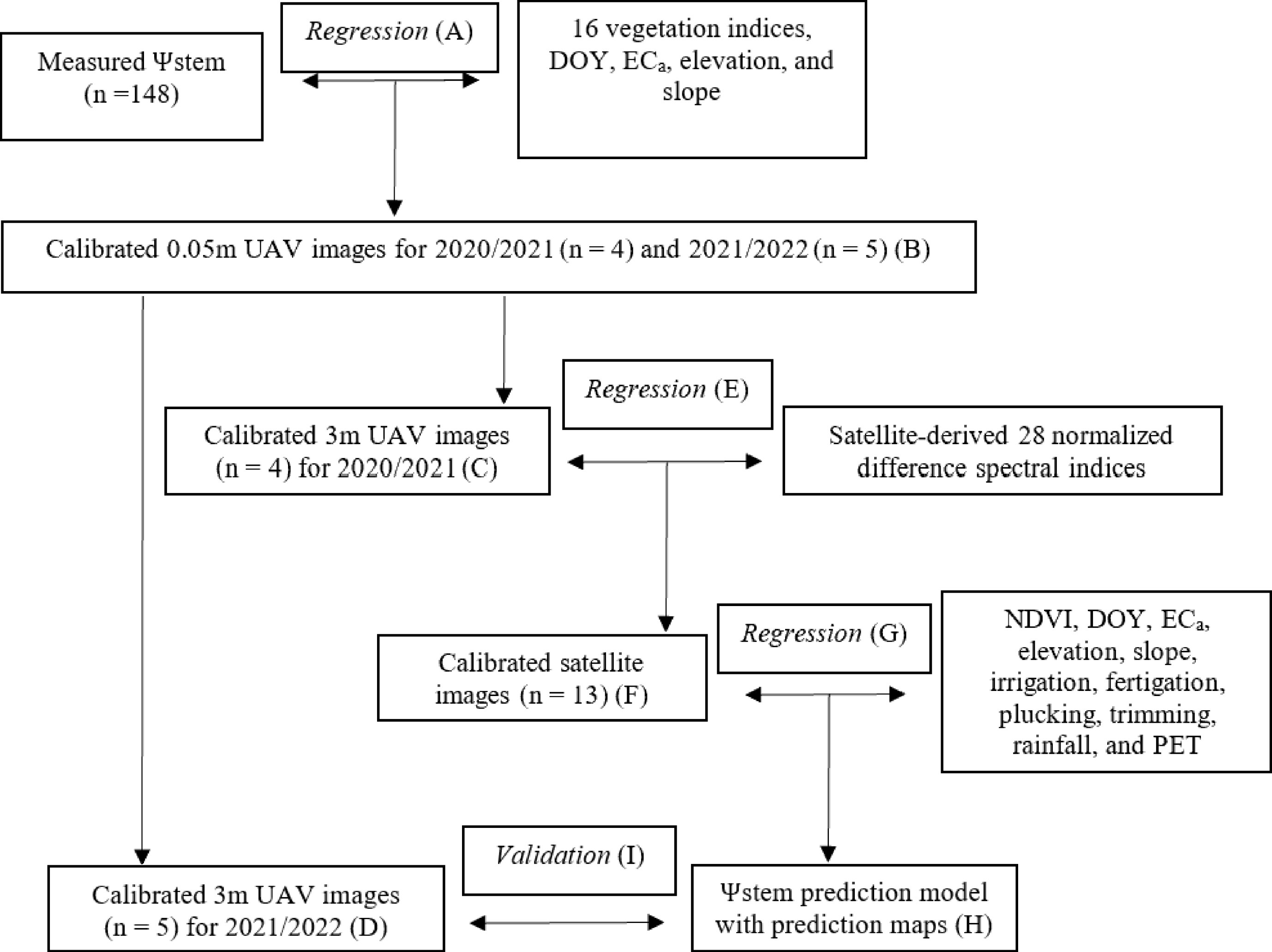
Figure 3.
Overview of the workflow. UAV = uncrewed aerial vehicle; DOY = day of the year; NDVI = normalized difference vegetation index; ECa = apparent electrical conductivity; PET = potential evapotranspiration.
Calibration of 0.05 m UAV images
-
Prior to the first calibration, models were developed by regressing the corresponding 16 VIs, DOY, ECa, elevation, and slope against measured Ѱstem data using RFR, SVR, and MLP (Fig. 3a). For each grapevine trunk position, the mean values of ECa, elevation, slope, and 16 vegetation indices based on the pure canopy pixels within 0.5 m distance of the trunk were computed for modeling. The acquisition of specific canopy pixels was carried out by overlapping the buffer zones (using recorded trunk location as the center of a circle with a radius of 0.5 m) with the binary raster of canopy height described previously.
The models with the best performance (in terms of RMSE on the test sets) were developed separately for the first growing season (2020/2021) and the second growing season (2021/2022). These models were then used to calibrate the UAV images acquired during 2020/2021 (n = 4) and 2021/2022 (n = 5) (Fig. 4a), respectively, to obtain calibrated UAV images exhibiting Ѱstem estimation across the vineyards at 0.05 m resolution (Figs 3b; 4b).
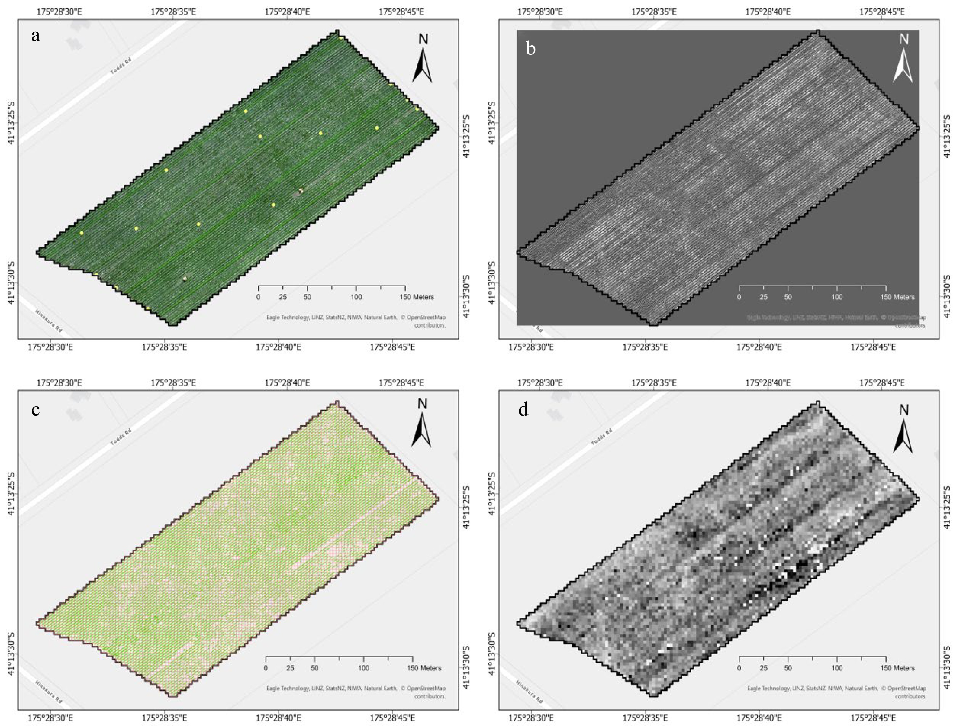
Figure 4.
An illustration of generating a downscaled 3 m UAV image for each UAV survey date. (a) UAV image is presented as RGB composites, with measured Ѱstem presented as yellow points. (b) Calibrated 0.05 m UAV image exhibiting Ѱstem estimation. (c) Green pixels are pure pixels representing grapevines after clipping pixels of interrow, overlaid with 3 m red grids. (d) Downscaled 3 m UAV image after spatial aggregation of pixels in red grids.
Generation of downscaled 3 m UAV images
-
To proceed with the second calibration for UAV-satellite image pairs (Table 1), image co-registration is an essential step. Since UAV images are more spatially accurate due to correction by ground control points, it is a good practice to register the PS images onto the UAV images. In ArcGIS Pro, the UAV images were first resampled from 0.05 m to 3 m resolution and were then used as reference images for the alignment of the PS images. All PS images were then re-aligned with the resampled 3 m UAV images using 'Snap Raster'. Grids of the 3 m pixels were generated by vectorizing the reference images using 'Raster to Point' and 'Create Thiessen Polygons'. As the pixel size of the PS images (3 m) was an integer multiple of that of the UAV images (0.05 m), every PS pixel corresponded to 3,600 UAV pixels after co-registration.
To remove the pixels that did not represent grapevines, the canopy polygons were created based on the binary raster of canopy height obtained previous using 'Raster to Polygon' for each UAV survey day. These canopy polygons were used to clip the corresponding calibrated UAV images obtained previously to acquire canopy pixels representing grapevines (Fig. 4c). Those UAV canopy pixels residing in the same cell of the 3 m grids were averaged using 'Spatial Join'. Nine downscaled 3 m UAV images (four images in 2020/2021 and five images in 2021/2022) were created (Fig. 3c & d); Fig. 4d). These downscaled UAV images, representing Ѱstem variability across the vineyards at 3 m resolution, served as references for the calibration of PS images in 2020/2021 (Fig. 3e) and for the validation of Ѱstem prediction in 2021/2022 (Fig. 3i).
Calibration of satellite images
-
For the second calibration, models were developed by regressing 28 normalized difference spectral indices (NDSIs) derived from every pixel of the PS images (n = 4; indicated by orange outlines in Table 1) against the reference Ѱstem values derived from the 3 m calibrated UAV images (n = 4) acquired in 2020/2021 using RFR, SVR, and MLP (Fig. 3e). NDSIs were computed using all possible pairwise-band combinations in the PS images using 'combinations' from the itertools package in Python. The UAV-satellite image pairs had at most one day apart in acquisition date to minimize spectral differences (Table 1). The developed models with the best performance (in terms of RMSE on the test sets) were used to calibrate all the PS images (n = 13) acquired during 2020/2021. The series of calibrated satellite images (Fig. 3f), representing Ѱstem estimation at 3 m resolution, was subsequently used as the response variable in the development of the Ѱstem prediction model.
Development of Ѱstem prediction model
-
Ѱstem prediction models were developed by regressing DOY, NDVI, ECa, elevation, slope, total daily rainfall, total daily PET, irrigation, fertigation, plucking, and trimming events, against the reference Ѱstem values derived from the calibrated satellite images (Fig. 3g). NDVI was selected because it is a widely used proxy for vegetation performance which can partially explain the variation in GWS[60]. The underlying assumption of the Ѱstem prediction model is that ECa, elevation, and slope are static during the growing seasons by taking advantage of the temporal stability in the spatial patterns of both NDVI and ECa[61,62]. NDVI needs to be collected at the beginning of each growing season. During any period in the growing season, managers then rely on weather forecasts for estimating total daily irrigation and PET as well as expected cultivation practices (including irrigation, fertigation, plucking, and trimming) to predict the variation of Ѱstem in vineyards.
NDVI, ECa, elevation, and slope were computed based on the pure canopy pixels within each cell of the 3 m grids. Total daily rainfall, total daily PET, irrigation, fertigation, plucking, and trimming on each day of the 30-day period before the date of Ѱstem prediction were used as independent predictors. Plucking and trimming events were noted using one-hot encoding (1 to mark the event and 0 if the event did not occur). The total number of predictor variables was 125 (Table 3).
Table 3. A summary for the predictors used in developing the Ѱstem prediction model. DOY = day of the year; NDVI = normalized difference vegetation index; ECa = apparent electrical conductivity; PET = potential evapotranspiration.
Predictor Note Number DOY The number is added on along the growing
season.1 NDVI Collected in late November for the 2020/2021 and 2021/2022 seasons separately. 1 ECa − 1 Elevation − 1 Slope − 1 Total daily rainfall The rainfall amounts on each day of the 30-day
period beforehand was used as a predictor.30 Total daily PET The PET amounts on each day of the 30-day
period beforehand was used as a predictor.30 Irrigation and
FertigationThe water input amounts, either sourced from
irrigation or fertigation, on each day of the 30-day period beforehand was used as a predictor.30 Plucking and Trimming The occurrence of the events on each day of the 30-day period beforehand was used as a
predictor.30 -
Both vineyards were visited nine times over two growing seasons, from flowering in late November to veraison in late January. Figure 5 displays the variability in Ѱstem collected from 148 canopies at the two vineyards, and the distribution of the measurements on each date. The maximum and minimum observation of Ѱstem is 1344 and 310 kPa in 2020/2021, and 1086 and 293 kPa in 2021/2022, respectively. Overall, there is an increasing trend of dehydration in GWS with time for both growing seasons, indicating the increasing presence of water deficit in the grapevines. The only exception is an increase in hydration on 9th December 2021 (compared to the previous measurement) due to rainfall events before sampling (i.e., 38.8 mm on 6th December 2021 and 11 mm on 7th December 2021). In Fig. 5, the height of the box (the difference between the upper quartile and lower quartile) represents the spatial variation of Ѱstem on one date across the relevant vineyard. This difference increased as the survey proceeded, implying spatial variation within the vineyards became more pronounced as water deficit increased. The mean values of Ѱstem obtained at Pencarrow were lower than those obtained at Wharekauhau on most of the measurement dates.
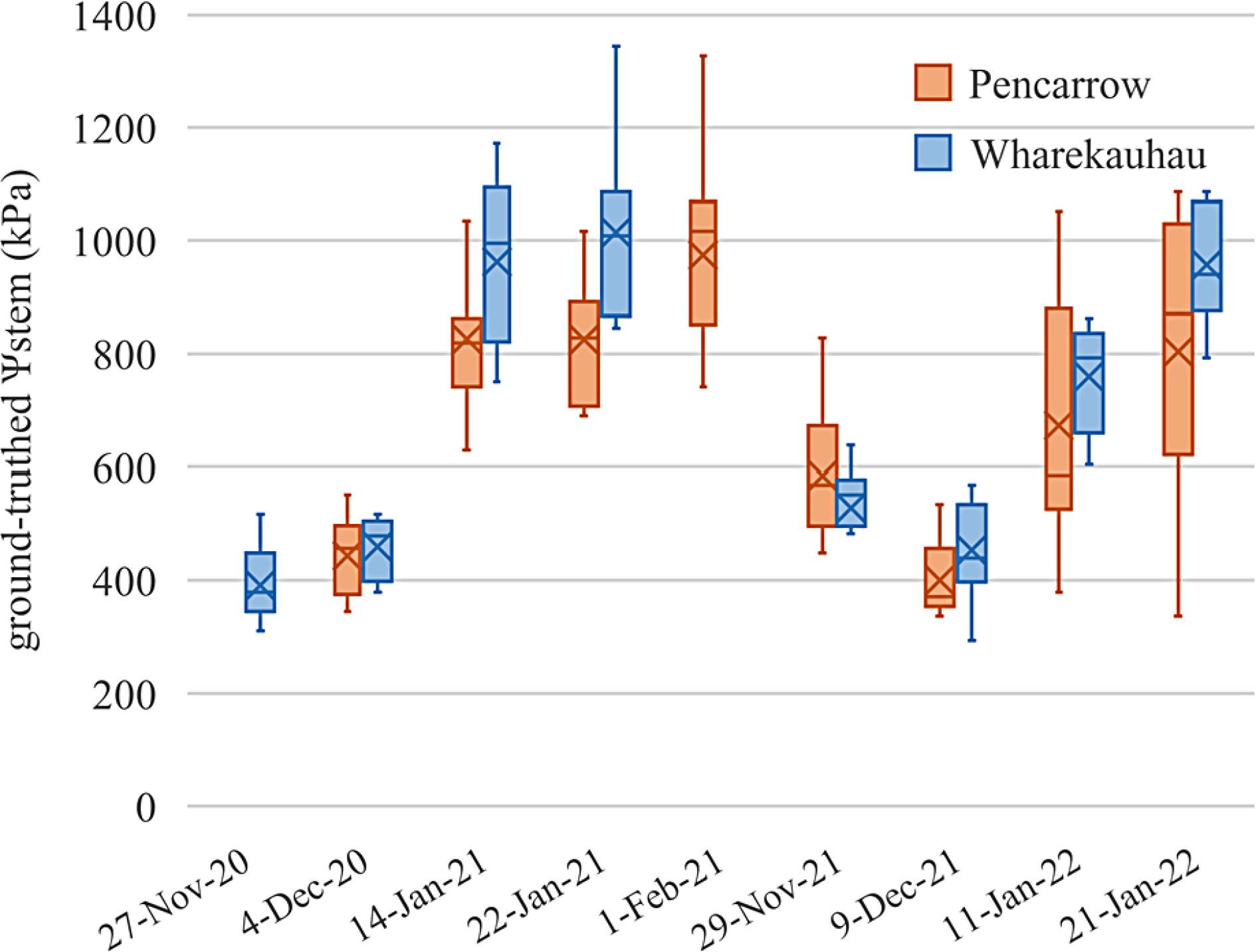
Figure 5.
Box plot of measured Ψstem collected during two growing seasons at Pencarrow (n = 86) and Wharekauhau (n = 62) vineyards. X symbols refer to the average values on the survey dates. Horizontal lines in the boxes refer to median values on the survey dates.
Modeling performance
-
The regression modeling was conducted for the two-stage calibration (Fig. 3a & e) and the development of the Ψstem prediction model (Fig. 3g) using RFR, SVR, and MLP. The ML models with the best performance (in terms of RMSE on the test sets) were chosen (Table 4). The RMSE of the test sets for two-stage calibration, ranging from 59 to 113 kPa, indicates that the estimation obtained from the calibration models is well correlated with measured Ψstem (first calibration) and reference Ψstem (second calibration; Fig. 3c). Therefore, the calibrated satellite images (Fig. 3f) should serve as a robust reference as response variables for Ψstem prediction (Fig. 3g). The RMSE of the test sets for Ψstem prediction is 31 kPa, suggesting the prediction model adequately captured Ψstem variability in 2020/2021. The scatter plots (Fig. 6) show that the data distribution for each regression model is closely clustered around the 1:1 line.
Table 4. Results of modeling performance. UAV = uncrewed aerial vehicle; Ψstem = stem water potential; RMSE = root mean square error.
Modeling purpose Regression model Data size of measured
or reference ΨstemRMSE of the
training set (kPa)RMSE of the
test set (kPa)Calibration of UAV images
acquired in 2020/2021
(Fig. 3a)Multilayer
perceptron85 96 113 Calibration of UAV images
acquired in 2021/2022
(Fig. 3a)Random forest
regression63 121 106 Calibration of
Satellite images (Fig. 3e)Random forest
regression42,234 47 59 Prediction of Ψstem (Fig. 3g) Random forest
regression151,580 25 31 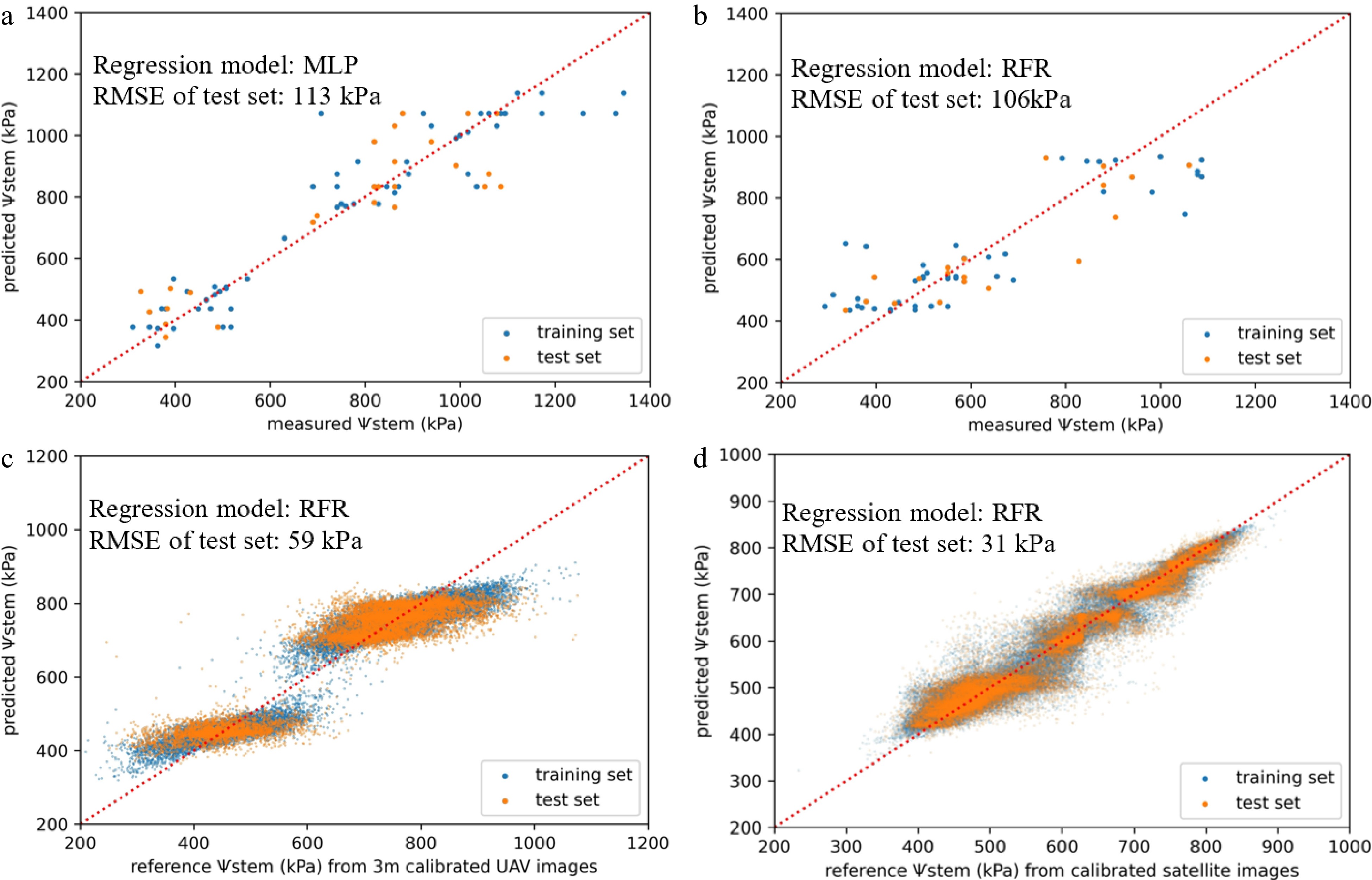
Figure 6.
Scatter plots between predicted Ѱstem and measured or reference Ѱstem (kPa) for the training and test sets of (a) the calibration of UAV images acquired in 2020/2021. (b) Calibration of UAV images acquired in 2021/2022. (c) Calibration of satellite (PS) images. (d) Prediction of Ѱstem in 2020/2021. Red dashed lines are 1:1 lines. Samples from the two study vineyards are considered collectively in each regression model.
The accuracy of the spatial and temporal patterns of Ψstem prediction
-
An important goal of this study was to validate whether a Ψstem prediction model based only on the first-season data (2020/2021) can be used to predict Ψstem changes in the second season (2021/2022). The similarity analysis, between Ψstem prediction maps (obtained from the best prediction model) and the Ψstem reference maps (obtained from 3 m calibrated UAV images in 2021/2022) was conducted using Pearson correlation for each vineyard. The values of r represent the degree of consistency between predicted and reference maps across multiple survey dates, with p-values showing a significant association (Table 5).
Table 5. Results of similarity analysis, presented by the Pearson correlation coefficient (r), represent the consistency between predicted and reference Ψstem maps across four survey dates for the two study vineyards.
Pencarrow Wharekauhau r 0.89* 0.87* Significance levels are noted as * when p ≤ 0.001. Figure 7 shows Ψstem prediction alongside measured Ψstem values (collected by grid sampling throughout the study periods in 2021/2022) during the season for both vineyards. Ψstem predictions were normalized for better visualization. Both Ψstem prediction series for both vineyards appear to intercept with each of the spreads of measured Ψstem data approximately at their average value, except for the last measurements at Wharekauhau vineyard. Note that higher Ψstem values indicate more dehydrated vines. Measured Ψstem values are assumed to represent the total variability of each vineyard. Thus, this result indicates that the temporal patterns in 2020/2021 captured by the Ψstem prediction model can provide good temporal predictions during the study period in 2021/2022.
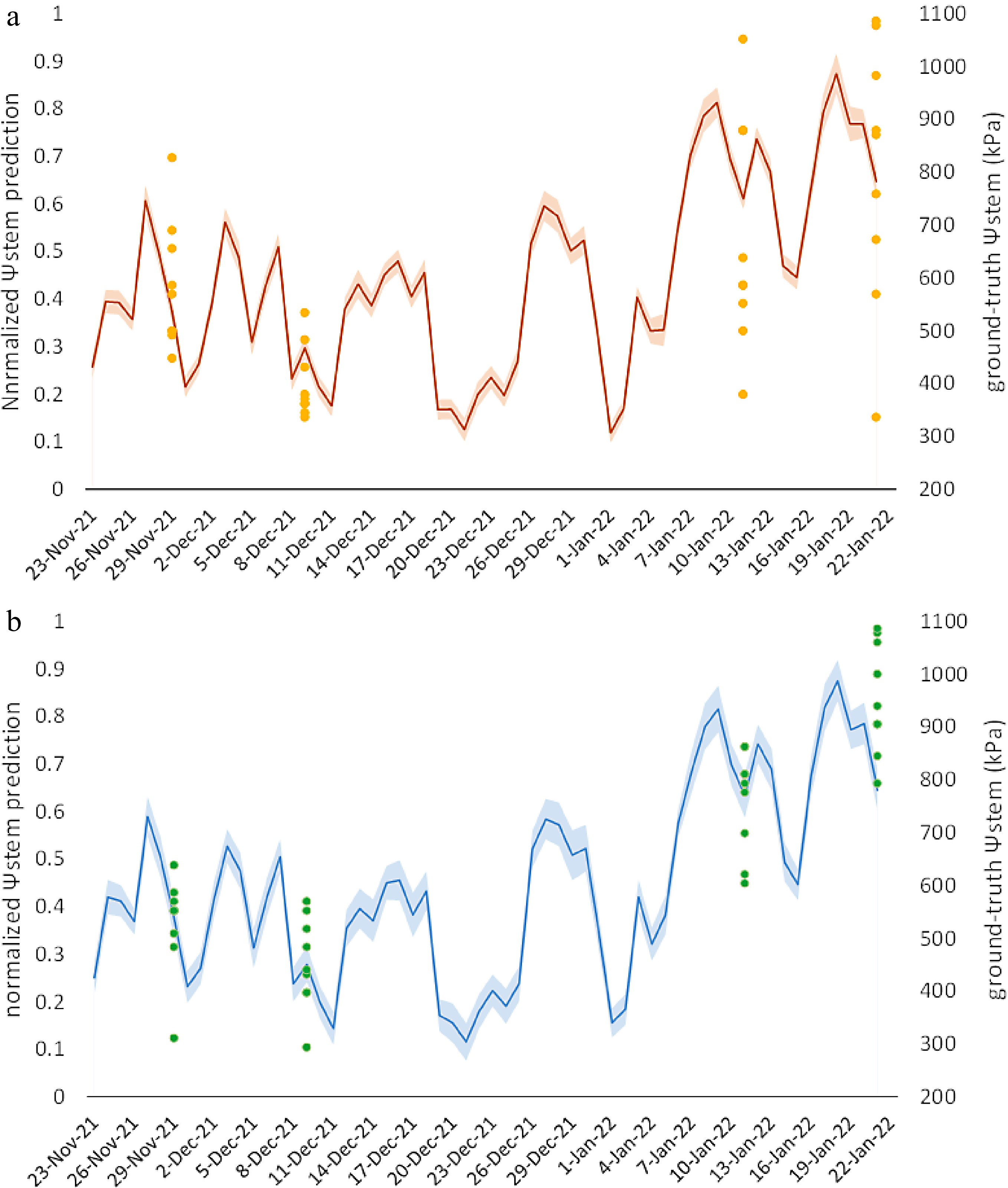
Figure 7.
The temporal patterns of normalized Ψstem prediction (lines) during the growing season in 2021/2022, with the measured Ψstem measurements (points) for (a) Pencarrow and (b) Wharekauhau. The shaded bands bordering the lines encompass one standard deviation.
Descriptive statistics, including mean, standard deviation (SD), and coefficient of variation (CV), are presented in Table 6 to help assess the 2021/2022 datasets of measured Ψstem values, reference Ψstem values obtained from 3 m calibrated UAV images, and predicted Ψstem values generated by the Ψstem prediction model. The statistics indicate that measured Ψstem values (CV > 10%) were more heterogeneous than the Ψstem values in the corresponding 3 m calibrated UAV datasets (4% > CV > 2%) and the prediction datasets (CV < 2%). Thus, the tendency to exhibit extreme Ψstem values decreases from the 3 m calibrated UAV datasets (n = 42,234, Ψstemmax = 867, Ψstemmin = 473) to the prediction datasets (n = 151,580, Ψstemmax = 694, Ψstemmin = 550) compared to the measured datasets (n = 63, Ψstemmax = 1,086 kPa, Ψstemmin = 293 kPa). Although there are differences in the absolute values and variability of Ψstem for the three datasets, they approximately follow the same temporal patterns over the study period in 2021/2022 (Fig. 8). This indicates that both 3 m calibrated UAV datasets and Ψstem prediction datasets are more reliable predictors of the temporal patterns of Ψstem, rather than their absolute values.
Table 6. Summary statistics for predicted Ψstem, Ψstem acquired from 3 m calibrated UAV images, and measured Ψstem for each survey date at the Pencarrow and Wharekauhau vineyards. UAV = uncrewed aerial vehicle; SD = standard deviation; CV = coefficient of variation.
Survey date Vineyard Data source Mean SD CV 29th November 2021 Pencarrow Predicted Ψstem 609 5.59 0.92 Ψstem from 3 m calibrated UAV 562 18.11 3.22 Measured Ψstem 585 113.93 19.47 Wharekauhau Predicted Ψstem 603 9.26 1.53 Ψstem from 3 m calibrated UAV 565 21.86 3.87 Measured Ψstem 528 87.31 16.55 9th December 2021 Pencarrow Predicted Ψstem 593 5.03 0.85 Ψstem from 3 m calibrated UAV 547 15.19 2.78 Measured Ψstem 400 64.25 16.05 Wharekauhau Predicted Ψstem 580 8.95 1.54 Ψstem from 3 m calibrated UAV 548 17.42 3.18 Measured Ψstem 453 82.18 18.14 11th January 2022 Pencarrow Predicted Ψstem 662 4.84 0.73 Ψstem from 3 m calibrated UAV 681 19.53 2.87 Measured Ψstem 672 204.27 30.39 21st January 2021 Pencarrow Predicted Ψstem 670 6.73 1.01 Ψstem from 3 m calibrated UAV 717 22.86 3.19 Measured Ψstem 803 233.27 29.03 Wharekauhau Predicted Ψstem 668 10.35 1.55 Ψstem from 3 m calibrated UAV 740 24.67 3.34 Measured Ψstem 957 99.35 10.39 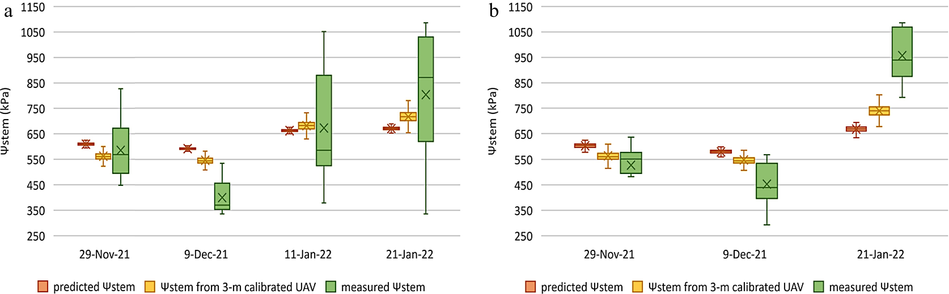
Figure 8.
Box plots of predicted Ψstem values, Ψstem values acquired from 3 m calibrated UAV images, and measured Ψstem values for each survey date at the (a) Pencarrow and (b) Wharekauhau vineyards. UAV = uncrewed aerial vehicle, and Ψstem = stem water potential.
-
To generate reference Ψstem data for subsequent prediction modeling, two-stage calibration was employed to calculate Ψstem data from satellite images based on measured Ψstem data using RFR, SVR, and MLP. Satellite images (obtained from PS in this study) have advantages over UAV data or measured data, in terms of higher coverage during one acquisition and regular acquisition periods. Therefore, satellite images are a better source in terms of providing observations on a regular basis. However, when assessing vertically-oriented grapevine status with discontinuous layouts, the utilization of low-to-moderate satellite resolution is often challenging due to the biased estimation resulting from pixels with mixed signals[10]. To address the issue of mixed-signal pixels, two calibration events were applied to scale the measured measurements up to data at the 3 m satellite level. UAV-based data served a critical role in this approach as it enhanced spectral purity by removing non-grapevine pixels and provided a large number of 0.05 m reference data, which was then spatially aggregated to ensure scale matching between satellite data and measurements[13,14]. The performance (in terms of RMSE on the test sets) of the first and the second calibration for the data acquired in 2020/2021 was 113 and 59 kPa, respectively (Table 4). These results supported the appropriateness of this two-stage calibration approach in generating large reference datasets (n = 151,580), compared to the measured samples (n = 85), for later modeling purposes.
Predicted Ψstem data generated by the Ψstem prediction model
-
The Ψstem prediction model was developed using calibrated PS images acquired in 2020/2021 as response variables, and using NDVI, ECa, elevation, slope, DOY, irrigation, fertigation, plucking, and trimming events, daily total rainfall, and daily total PET as predictors. The need for this Ψstem prediction model was demonstrated by the number of PS acquisition images in this study. As the revisit period of PS is daily, there should potentially be 80 images, with surface reflectance assets, proper ground control, and standard quality, available over the study periods during 2020/2021 (15th November 2020 to 2nd February 2021). Nevertheless, there were only 20 images available to download, with only 13 images (the longest time gap between acquisition dates being 17 d) suitable for analysis (after eliminating those images contaminated with cloud, haze, or cloud shadow). Bellvert et al.[63] have suggested access to five to six points of information acquisition over the season for vineyard irrigation scheduling when considering cost efficiency. To avoid inaccessible satellite data caused by weather or technical problems, the development of a GWS prediction model is desirable.
The trained model performed well on the test set of data obtained in 2020/2021, with an RMSE of 31 kPa on the test sets (Table 4). From the two-stage calibration to Ψstem prediction, it appears the accuracy of modeling was higher as the data size of measured or reference Ψstem increased, resulting from the two-stage calibration. This confirmed that ML models develop more robust relationships with fewer overfitting issues when they are trained with more samples[64]. The superior performance of RFR with calibration and prediction modeling is probably because RFR is robust to multicollinearity[65]. Multicollinearity was evident in the datasets of this study, originating from VI computation based on the same spectral band, and temporal autocorrelation between the rainfall and PET data series.
In this study, the model was further evaluated with the data independently collected during a second growing season (2021/2022) to test its generalization performance. The model reflected the trends of changes of Ψstem in response to measured Ψstem. The predicted temporal patterns became more hydrated in early December compared to late November but exhibited increasing water deficit as the growing season proceeded, which is comparable to measured Ψstem data (Figs 5 and 7). Similarity analysis (in terms of r) indicated that temporal patterns were well depicted by the prediction models for both vineyards (Table 5). It should be noted that the model’s prediction capability was evaluated using calibrated UAV images (reference maps) instead of using measured Ψstem. The reason for this is the output of the prediction model is 3-m spatial resolution, and each pixel corresponds to multiple grapevines. Thus, the outputs cannot be directly compared with individually measured Ψstem. Besides, PS images acquired in 2021/2022 cannot be used for evaluation because background information (soil and grass) is included. Therefore, the prediction model was evaluated using the calibrated UAV images that approximated the measured Ψstem assumed to represent the total GWS variability across the study vineyards (RMSE = 106 kPa). The results of similarity analysis may be attributed to the observed similarity in PET variability over the two seasons (Fig. 2). As ET is a critical component in the soil water balance contributing to Ψstem[66], the similarity of ET from different seasons may lead to a similarity in the temporal variation of Ψstem over different years. Another reason for the similarity is that cultivation practices were applied within similar timeframes during each growing season, so their impacts were still within the prediction range of the model. In addition, both NDVI-defined and ECa-defined zones have been reported to support spatial assessment of GWS[58,67], further increasing the prediction capabilities of the model.
The prediction model established the temporal variation of Ѱstem based on DOY, 30-day total daily rainfall, 30-day total daily PET, 30-day irrigation, 30-day fertigation, 30-day plucking, and 30-day trimming, while accounting for the spatial variation of Ѱstem based on NDVI, ECa, elevation, and slope. Although temporal patterns of Ѱstem were tested with promising results, it should be noted that the relative pattern of values, rather than their absolute values, should be the focus of attention in this study. Therefore, sampling for Ψstem prediction should be undertaken at the beginning of each growing season for model calibration, so as to enhance the precision and practicability of the model for use in irrigation scheduling.
Limitations and directions for future research
-
The weakness of the prediction model in this study lies in its empirical approach, so it is unable to provide a reliable prediction if the inputs are beyond the range of observed variability. Field measurements are needed to validate the prediction model with data collected from additional phenological stages, growing seasons, and sites, to enhance the model’s scope. In addition, due to the selection of 3 m resolution satellite images, high heterogeneity of GWS within a cell of grids would be averaged and exhibit less variation in Ψstem, thus introducing bias into calibration and modeling.
In its current form, this prediction model will only be able to predict Ψstem at vineyard-block scale during the growing season, rather than provide a spatial map of Ψstem each day. One reason is that weather predictors (including daily total rainfall, and daily total PET) were assumed to be evenly spatially distributed across the two vineyards. Predictors accounting for spatial variation (including NDVI, ECa, elevation, and slope) are static during modeling and are determined before the growing seasons. Despite these limitations, this prediction model is still a potentially practical tool for viticulturists since the block size of the results can be adjusted, by increasing the number of weather sensors or stations, to suit the size of zones that need different irrigation management.
Subsequent research is suggested to explore new predictor variables that are cost-effective to acquire and can serve as spatio-temporal proxies for Ψstem. Weather parameters, recorded spatially and continuously by wireless sensor networks across vineyards, could be one of these potential predictors. Further research work should examine the number and type of field measurements required and protocols needed for vineyard sampling to contribute to model calibration at the beginning of the growing season. The impact of the quality of weather forecasts on the performance of the prediction model also requires investigation. This will, potentially, allow the model to become a more reliable prediction tool, providing daily Ψstem spatial maps in advance throughout the growing season.
-
This study demonstrated the potential application of using a two-stage calibration approach for calibrating satellite images to provide reference stem water potential (Ψstem) data. The potential of establishing a Ψstem prediction model based on day of the year, normalized difference vegetation indices, apparent electrical conductivity, elevation, slope, rainfall, potential evapotranspiration, irrigation, fertigation, plucking, and trimming events, was also demonstrated. Collection of ground truthing is required for model calibration at the beginning of the growing season. The prediction model can be improved on a daily basis if predictors that account for spatio-temporal variability in Ψstem are provided, such as spatially recorded weather information. This tool has the potential to benefit vineyard managers with improved irrigation management and quality optimization by providing Ψstem predictions at vineyard-block scale during growing seasons, when the model is properly calibrated and coupled with accurate weather forecasts.
This study was funded by a grant from the Massey University Research Fund (MURF) and a grant from the New Zealand Horticulture Trust. The authors sincerely thank Palliser Estate for providing the vineyards as study fields, and Guy McMaster (chief viticulturist of Palliser Estate) for offering the pressure chamber during the research period. Additional thanks are given to New Zealand eScience Infrastructure (NeSI) for providing the platform of high performance computing for the use of modeling and data analysis.
-
The authors declare that they have no conflict of interest.
- Copyright: © 2023 by the author(s). Published by Maximum Academic Press, Fayetteville, GA. This article is an open access article distributed under Creative Commons Attribution License (CC BY 4.0), visit https://creativecommons.org/licenses/by/4.0/.
-
About this article
Cite this article
Wei HE, Grafton M, Bretherton M, Irwin M, Sandoval E. 2023. Evaluation of the use of two-stage calibrated PlanetScope images and environmental variables for the development of the grapevine water status prediction model. Technology in Agronomy 3:6 doi: 10.48130/TIA-2023-0006 

Evaluation of the use of two-stage calibrated PlanetScope images and environmental variables for the development of the grapevine water status prediction model
- Received: 07 December 2022
- Accepted: 19 April 2023
- Published online: 02 June 2023
Abstract: Grapevine water status (GWS) assessment between flowering and veraison plays an important role in viticulture management in terms of producing high-quality grapes. Although satellites and uncrewed aerial vehicles (UAV) have successfully monitored GWS, these platforms are practically limited because data transfer is delayed due to post processing and UAV operation is weather dependent. This study focuses on addressing two issues: the unreliability of GWS estimation using satellite images with low-moderate spatial resolution and the inaccessibility of real-time satellite data. It aims to predict the temporal variation of GWS based on a prediction model using spectral information (calibrated PlanetScope (PS) images), soil/topography data (apparent electrical conductivity, elevation, slope), weather parameters (rainfall and potential evapotranspiration), cultivation practices (irrigation, fertigation, plucking, and trimming), and seasonality (day of the year) as predictors. Stem water potential (Ψstem) was used as a proxy for GWS. Two-stage calibration, including an initial calibration of UAV images with measured Ψstem and a subsequent calibration of satellite images with calibrated UAV data, was applied to calibrate the PS images. Three machine learning models (random forest regression, support vector regression, and multilayer perceptron) were used in the calibration and modeling process. The results showed that a two-stage calibration can generate reliable reference data, with a root mean square error of 113 kPa and 59 kPa on the test sets during the first and second calibration stage, respectively. The prediction model described the temporal variation of block Ψstem when compared with the measured Ψstem. In the similarity analysis, the Pearson correlation coefficient was 0.89 and 0.87 between predicted and reference Ψstem maps across four dates for the two study vineyards. This study supports the concept of developing an approach to predict grapevine Ψstem, which would enable growers to acquire Ψstem variation in advance during the growing season, leading to improved irrigation scheduling and optimal grape quality.
-
Key words:
- Satellite /
- UAV /
- Stem water potential /
- Random forest regression /
- Support vector regression /
- Multilayer perceptron