










-
With the acceleration of urbanization and the continuous growth of travel demand, large metropolitan areas have become increasingly dependent on efficient and reliable bus systems. Public transportation plays a vital role in mitigating traffic congestion, reducing environmental pressure, and promoting sustainable urban development. However, real-world bus operations still face several inefficiencies, including excessively long routes, uneven passenger distribution, and high station density. These factors often result in unnecessary dwell times, boarding delays, and reduced service reliability. To improve operational efficiency, many major cities in Europe and North America began to adopt skip-stop bus operations in the twentieth century. By skipping stations with relatively low demand, this strategy reduces the number of stops, shortens passenger travel time, and alleviates congestion at busy stations.
The outbreak of COVID-19 in 2020 further exposed the vulnerability of public transportation systems during public health emergencies. Enclosed vehicle environments, limited ventilation, and high passenger density significantly increased the risk of airborne disease transmission. Empirical studies indicate that bus ridership in Budapest declined by approximately 80% during the pandemic, while Switzerland experienced a decline exceeding 90%. In China, metro ridership exhibited a strong negative correlation with the number of newly confirmed cases within short time periods[1−4]. These observations highlight that bus operations must consider not only efficiency but also passengers' exposure risk and overall health safety to maintain system resilience during pandemics and seasonal infectious disease outbreaks.
To address the high-contact nature of bus operations and potential infectious disease risks, this study investigates a cyclic skip-stop bus scheduling problem that integrates epidemic exposure risk into operational decision-making. We develop an integrated optimization model that simultaneously considers station-level risk indicators, cumulative in-vehicle exposure, and passenger travel time, enabling scheduling decisions to balance operational efficiency and health risk. To solve this complex multi-layer, multi-constraint combinatorial problem, we design an Adaptive Large Neighborhood Search algorithm and propose a set of risk-aware scheduling strategies validated on real-world bus operation data, suitable for post-pandemic safe transit operations.
In this work, COVID-19 is considered a representative example of respiratory infectious diseases. Based on the risk modeling insights derived from COVID-19, the proposed framework is extended to more general respiratory and airborne infectious diseases, including seasonal and emergency public-health scenarios. Station-skip operations were originally introduced to improve operational efficiency by reducing ineffective stops, increasing route speed, shortening in-vehicle travel time, and lowering cumulative close-contact duration among passengers. These operational objectives are closely aligned with infection risk mitigation. Therefore, station-skip decisions are incorporated as the primary scheduling mechanism through which passenger contact levels, cumulative in-vehicle exposure risk, and travel efficiency are simultaneously evaluated and optimized, making station-skip the central decision variable of the model.
The main contributions of this study are:
(1) Joint optimization of epidemic exposure risk and traditional bus scheduling metrics, achieving a balance between passenger health and operational efficiency;
(2) Dynamic cumulative risk modeling, which quantifies the accumulation of exposure risk as passengers remain onboard, enabling fine-grained evaluation of scheduling decisions;
(3) Development of an ALNS algorithm and risk-aware scheduling strategies for the cyclic skip-stop problem, capable of efficiently solving the multi-objective, multi-constraint combinatorial problem and providing scalable, high-quality solutions suitable for large-scale bus operations.
-
In recent years, the rapid advancement of big data, artificial intelligence, and optimization algorithms has led to remarkable progress in the research of bus scheduling optimization. Over the past decades, models and solution technologies in public transit systems have experienced significant development, further underscoring the importance of continuous innovation in this domain. Guihaire & Hao[5] undertook a thorough examination of the pivotal strategic and tactical considerations in public transport planning. The operational planning of public transport encompasses multiple sequential steps, including: (1) the design of network routes; (2) the development of schedules; (3) the allocation of vehicles; and (4) the scheduling of personnel. Bus scheduling optimization holds the utmost significance within public transport planning.
The fundamental iteration of the Vehicle Scheduling Problem (VSP) is the Single Station Single Type Vehicle Scheduling Problem, which aims to establish a schedule ensuring that all trips are served by vehicles originating from and returning to the same station. Freling et al.[6] and Bunte & Kliewer[7] introduced several models and algorithms for single-station vehicle scheduling, reporting significant performance improvements in computation time. Another variant of the VSP is the multi-site vehicle scheduling problem, where vehicles may depart from different locations. This assumption leads to more intricate representations, such as the multi-commodity network flow model introduced by Bertossi et al.[8]. They also proposed the deficit function (DF), rooted in information graphics technology, to address multi-station VSP scenarios. The DF indicates insufficient vehicle quantities required at terminals within a multi-station network.
Liu & Ceder[9,10] utilized the DF method to develop a bilayer integer programming model for bi-objective scheduling. Based on the dual-layer structure of the model, they further proposed a DF-based sequential search method combining network flow and departure-time adjustment techniques to obtain Pareto-efficient solutions. Tang et al.[11] introduced a DF method aimed at reducing the required vehicle fleet through limited docking, idling, and hybrid strategies. This approach enables dispatchers to select flexible scheduling strategies based on application scenarios. Additionally, two optimization models were formulated to minimize passenger travel time while determining stations that can be effectively served by variable travel schedules.
Studies on multiple routes have mainly focused on transfer waiting times. Ibarra-Rojas & Muñoz[12] considered bus speed and arrival-time deviations and applied a genetic algorithm to generate coordinated schedules for overlapping segments of multiple routes. Shen & Du[13] sought to increase transfer availability between two bus lines by coordinating arrival times through unequal headway schedules, aiming to minimize total transfer waiting time. Song & Zhang[14] designed a bus query system using a minimum-transfer algorithm and conducted experimental analyses. Lu et al.[15] considered interactions among bus lines on passenger route choice and proposed coordinated multi-route flexible scheduling during off-peak hours.
Common operational control strategies include station-skipping[16−20], temporary parking at designated stops[21−25], and rescheduling[26−30]. Several studies have combined skipping and controlled stopping strategies[31−34]. Moreover, Gavriilidou & Cats[35] proposed a genetic algorithm based on the concept of virtual lines, recommending short-turning and hybrid control schemes. Gkiotsalitis & Maslekar[36] further introduced a stochastic optimization method for rescheduling and stop-based holding control. Cortés et al.[37] combined short-turning with temporary stop closures.
Passenger-oriented bus scheduling models
-
Lu et al.[15] analyzed how bus line interactions influence passenger route choice and proposed coordinated multi-route flexible scheduling during off-peak periods. He et al.[18] constructed a model to optimize real-time scheduling based on transfer passenger flow and system-wide minimum cost. Li et al.[19] developed multi-objective optimization models for coordinated multi-route scheduling to maximize social and enterprise benefits and designed a hybrid genetic tabu algorithm to solve them. Subsequently, Mazloumi et al.[21] formulated a scheduling method based on actual passenger-flow data and solved it with genetic algorithms and ant colony optimization. Zheng et al.[22] optimized customized shuttle bus service areas using a spatiotemporal accessibility model solved by an improved tabu search algorithm. Furthermore, Deng et al.[23] introduced a real-time speed control model aimed at minimizing headway variations and analyzed its performance under various road infrastructure scenarios.
Skipping stops increases inconvenience for passengers who cannot board buses that skip their stations[38]. Holding buses at stops may also reduce passenger comfort due to additional delays. The main challenge for high-frequency service (HF) is to maintain scheduled headways at each stop[39], while the critical issue for low-frequency service (LF) is to maintain planned arrival times[40,41]. If the demand and travel times for all buses on a route are stable, headways remain uniform across downstream stations, resulting in regular service that aligns actual waiting times with passenger expectations.
Epidemic transmission modeling in transportation systems
-
The emergence of new infectious diseases over the past decade has heightened global concern, as predicting and controlling outbreaks remains a major public health challenge. Arthur Ransome, who first described the cyclical behavior of measles, developed a discrete-time epidemic model for cholera transmission in 1906[42]. His model addressed population-level dynamics and assumed homogeneous populations. Classical epidemic models divide host populations into compartments, where individuals interact with neighbors. The simplest model, the susceptible infectious removed (SIR) model, was proposed by Kermack & McKendrick[43] to describe disease spread in a closed population.
The spatiotemporal nature of transmission and heterogeneity across communities plays a significant role in designing public health interventions[44]. With advancements in computing and increased availability of spatiotemporal disease data, various modeling approaches have emerged to describe individual-level behaviors[45]. Statistical models, network-based models, and individual-based simulation approaches incorporate key causal factors such as individual mobility, social interactions, and contact patterns. Individual-based models are especially flexible in capturing heterogeneity in transmission and can incorporate spatial factors such as the influence of transport systems.
Various epidemic models have been developed to simulate transmission dynamics[46−48]. The COVID-19 outbreak exposed the limitations of existing modeling frameworks, particularly regarding transportation's role during outbreak emergence and response. According to Peeri et al.[49], globalization accelerated the spread of COVID-19. Wu et al.[50] argued that the proximity of the outbreak to the Chinese New Year and increased rail accessibility facilitated transmission. Modern transportation systems have intensified person-to-person contact, increasing transmission likelihood due to close proximity among travelers. To control the spread of COVID-19, governments worldwide implemented widespread suspensions of transportation networks[1−4].
-
With the objective of minimizing both the average passenger journey time and the risk of infection, this paper introduces a risk-sensing approach. Specifically, we focus on a one-way bus route system, where S = {1, 2, ..., |S|} represents the set of bus stations, and K = {1, 2, ..., |K|} denotes the collection of buses operating on a circular jump station scheduling scheme. Given the number of service cycles K, the maximum number of jump stations permitted, and the designated number of jump stations for each bus, the objective is to determine the optimal station s
$\in $ Table 1. Notations, input parameters, and variables.
xxx Set S = {1, 2, ......, |S|}, represents a set of bus stops K = {1, 2, ......, |S|}, represents a set of vehicles within a service cycle Parameter ti The running time of public transportation from the i-th station to the i + 1st station P The duration of time that buses spend at each stop hmin The minimum safe time interval, known as the headway, that must be maintained between adjacent buses running on the same route hmax The maximum safe time interval, known as the headway, that must be maintained between adjacent buses running on the same route C The capacity of a bus, which typically refers to the maximum number of passengers it can safely transport β Input parameter to estimate the average waiting time for passengers at a bus stop who are anticipating the arrival of the next bus that can take them to their destination Decision variable $ x_{i}^{k} $ 0,1 variable, if K car stops at station i, take 1; otherwise, take 0 $ y_{ij}^{k} $ 0,1 variable, if the k-car stops at both i and j stations, take 1; otherwise, take 0 Intermediate variable $ {h}_{L} $ The regular interval of time between the arrivals of consecutive buses at a given stop or along a route $ A_{i}^{k} $ The precise moment when train K reaches station i, within a given operational schedule $ C_{i}^{k} $ The maximum number of passengers that can board the k train when it stops at station i Passenger related parameters and variable parameters $ {\lambda }_{ij} $ The number of passengers from station i to station j per unit time $ {u}_{i} $ Static risk rating of passengers boarding at station i Intermediate variable $ d_{ij}^{k} $ The number of passengers who want to board the K train from station i to station j when it stops $ r_{ij}^{k} $ The number of passengers who want to travel from station i to station j before the arrival of train K $ r_{i}^{k} $ The total number of waiting passengers at station i before the arrival of train K $ R_{ij}^{k} $ The number of passengers who may board the K train at station i and go to station j $ R_{i}^{k} $ The total number of people who may board the K train at station i $ b_{ij}^{k} $ The actual number of people boarding the K train at station i to go to station j $ b_{i}^{k} $ The total number of people actually boarding the K train at station i $ w_{ij}^{k} $ The number of passengers who are stranded at station i and want to go to station j after the departure of train k $ n_{i}^{k} $ The total number of passengers inside the train k after leaving the station i Decision variable $ D_{i}^{k} $ The total risk inside the vehicle at station i $ Q_{i}^{k} $ Risk of infection among passengers in the train upon arrival at station i Pre-skip protection mechanism
-
Before implementing station-skip decisions, passenger boarding and alighting information is assumed to be known in advance through IC-card records, stop-request systems, or OD demand estimation. Under this pre-skip protection mechanism, a station is allowed to be skipped by a bus only if no passenger on board intends to alight at that station. Once a station is associated with any alighting demand for a given vehicle, it is marked as non-skippable for that vehicle. This mechanism ensures that all passengers can complete their intended trips without forced detours or missed alighting stops, while preserving the operational feasibility of station-skip scheduling.
Precise mixed-integer programming model
-
The objective of this study is to maximize the total reduction in passenger travel time within a service cycle (i.e., minimize total travel time) while simultaneously minimizing the cumulative infection risk of passengers. These two goals are balanced using weight parameters ω1 and ω2. The total travel time reduction ΔT is calculated as the difference between the reduction in on-board travel time due to station skipping (
$ {\Delta }{T}_{riding} $ $ {\Delta }{T}_{waiting} $ $ Maximize \;H={\omega }_{1}\Delta T-{\omega }_{2}\sum\nolimits_{i=2}^{\left| S\right| }{Q}_{i} $ (1) where,
$\begin{split}\Delta T=&\Delta {T}_{riding}-\beta \cdot \Delta {T}_{waiting} = \sum\nolimits_{k=1}^{\left| K\right| }\sum\nolimits_{i=2}^{\left| S\right| -1}n_{i-1}^{k}\cdot p\cdot \left(1-x_{i}^{k}\right)\\ &-\beta \cdot \sum\nolimits_{k=1}^{\left| K\right| }\sum\nolimits_{i=2}^{\left| S\right| -1}w_{i}^{k} \end{split} $ (2) Specifically, for each bus k, ni−1k represents the number of passengers on board after leaving the previous station, p represents the service time at a station, and xik equals 1 if the bus stops at station i, and 0 otherwise. If the bus stops at a station, the reduction in travel time for on-board passengers is zero. wik represents the number of passengers remaining at station i after bus k departs, and β is the estimated average waiting time at stations. Qi represents the cumulative i infection risk of passengers on board when the bus arrives at station i.
It should be noted that the objective of this model is infection risk minimization, rather than complete infection blocking. Completely blocking infection risk would require explicitly disconnecting all potential transmission paths in the network structure, resulting in a much more restrictive feasible region and substantial efficiency loss in public transit operations. In contrast, the proposed risk minimization framework allows a certain level of exposure but penalizes infection risk through a continuous, time-accumulative risk variable, which is jointly optimized with passenger travel time savings. This modeling choice is more consistent with the operational reality of routine bus services and with the characteristics of airborne disease transmission in enclosed vehicle environments.
Risk constraints
-
$ D_{i}^{k}=\sum\nolimits_{i=1}^{\left| S\right| }{u}_{i}\cdot b_{i}^{k}\;\;\forall k\in K $ (3) $ Q_{1}^{k}=0\;\;\forall k\in K $ (4) $ Q_{i}^{k}=Q_{i-1}^{k}+D_{i-1}^{k}({t}_{i-1}+p.x_{i}^{k})\;\;\forall i,\;j\in S,\;k\in K $ (5) $ 0 \lt Q_{i}^{k} \lt {Q}_{\max}\;\;\forall i,\;j\in S,\;k\in K $ (6) First, for each station i, we define a static risk factor ui, which characterizes the potential exposure risk arising from local passenger density, ventilation conditions in the waiting area, and other related factors. According to constraint (3), the risk increment at station i, denoted as Dik, is determined by the product of the static risk ui and the number of boarding passengers bik. This formulation reflects the marginal contribution of boarding behavior at each station to the overall in-vehicle risk level.
For cumulative risk calculation, constraints (4) and (5) specify that the cumulative risk of each bus is initialized to 0 at the first station. As the bus moves along the route, the in-vehicle risk gradually accumulates according to travel time and dwell time, causing the cumulative exposure risk Qik to increase continuously over time. This time-dependent accumulation is consistent with the fundamental mechanism of airborne disease transmission, in which infection risk typically increases as a linear or nonlinear function of exposure duration. Accordingly, the cumulative risk used in this study can be viewed as a simplified form of a time-dependent exposure model.
To prevent unrealistic unlimited growth, constraint (6) imposes an upper bound Qmax on cumulative risk, which captures the mitigating effects of vehicle ventilation, natural viral decay, and other preventive measures. Since viruses can remain suspended in the air for extended periods, modeling and observational studies of public transit and other enclosed transport environments indicate substantially elevated transmission risk compared with outdoor settings. For example, mathematical assessments of commuter trains and buses report markedly increased inhalation exposure under crowded and poorly ventilated conditions[51]. These findings support the use of a cumulative exposure-risk indicator in our model. Furthermore, the conceptual basis of cumulative airborne risk is consistent with the classical Wells–Riley framework for airborne infection, which provides a theoretical foundation for time-dependent exposure accumulation[52].
Fast vehicle service constraints
-
$ \sum\nolimits_{k=1}^{\left| K\right| }x_{i}^{k}\geq 1\;\;\forall i\in S $ (7) $ x_{1}^{k}=x_{\left| S\right| }^{k}=1\;\;\forall {k}\in {K} $ (8) $ y_{ij}^{k}=x_{i}^{k}\cdot x_{j}^{k}\;\;\forall {i},\;j\in S,\;k\in K $ (9) $ \sum\nolimits_{k=1}^{\left| K\right| }y_{ij}^{k}\geq 1\;\;\forall i,\;j\in S $ (10) $ x_{i}^{k}\in \left\{0{,}\;1\right\} $ (11) $ y_{ij}^{k}\in \{0{,}\;1\} $ (12) Constraint (7) states that each station is served at least once within a single service cycle. Constraint (8) specifies that all trains depart from and serve the first station (i = 1) and terminate their services at the last station (i = |S|), where |S| represents the total number of stations. Constraint (9) ensures that passengers can only be transported from one station to another if the train stops at both the boarding and alighting stations. Constraint (10) ensures that, within a service cycle, at least one train stops at both stations i and j, ensuring that all passengers can reach their destinations. Constraint (9) and (10), together with the pre-skip protection mechanism described in the problem definition, guarantees that every origin–destination pair is served by at least one feasible stopping pattern within a service cycle. Constraints (11) and (12) define the range of decision variables.
Headway time constraint
-
$ A_{1}^{1}=0 $ (13) $ A_{i}^{k}=A_{1}^{k}+\sum\nolimits_{i=1}^{i-1}{t}_{i-1}+p\cdot \sum\nolimits_{i=1}^{i-1}x_{i}^{k}\;\;\forall i\in S\backslash \{1\},\;k\in K $ (14) $ {h}_{\min}\leq A_{i}^{k+1}-A_{i}^{k}\leq {h}_{\max}\;\;\forall i\in S,\;k\in K\backslash \{\left| K\right| \}~ $ (15) Constraint (13) sets the arrival time of the first vehicle (k = 1) at the departure station to 0. Constraint (14) calculates the arrival time of each vehicle. Constraint (15) ensures that adjacent vehicles maintain a safe headway time and prevent overtaking.
Capacity Constraint
-
$ c_{1}^{k}=C\;\;\forall k\in K $ (16) $ c_{i}^{k}=C-n_{i-1}^{k}+\sum\nolimits_{j=1}^{i-1}b_{ji}^{k}\;\;\forall i\in S\backslash \{1,\;\left| S\right| \},\;j\in S,\;j \lt i,\;\forall k\in K $ (17) $ n_{1}^{k}=b_{1}^{k}\;\;\forall k\in K $ (18) $ n_{i}^{k}=n_{i-1}^{k}-\sum\nolimits_{j=1}^{i-1}b_{ji}^{k}+\sum\nolimits_{j=i+1}^{\left| S\right| }b_{ij}^{k}\;\;\forall i\in S\backslash \{1,\;\left| S\right| \},\;\forall k\in K $ (19) Constraints (16) and (17) represent the maximum number of passengers allowed to board a train. Constraints (18) and (19) calculate the relationship between the number of passengers on the train and the number of passengers boarding.
Passenger boarding and alighting constraints
-
Constraint (20) calculates the number of passengers who want to board the train for the trip from station i to station j. Constraint (21) defines how to calculate the number of stranded passengers at station i before train k arrives. The stranded passengers for trip OD i-j equal the number of arrivals within the interval plus the number of passengers who were unable to board the previous train. Constraint (22) states that the total number of stranded passengers is equal to the sum of all destination passenger counts. Constraints (23) and (24) calculate the potential boarding passengers. Only when the current train k stops at both the boarding and alighting stations can stranded passengers be converted into potential boarding passengers. Due to the capacity limitations of the bus, not all potential boarding passengers R may be able to board, so we introduce a binary variable θ to indicate whether all passengers board the train.
$ d_{ij}^{k}={\lambda }_{ij}\cdot \left(A_{i}^{k}-A_{i}^{k-1}\right)\;\;\forall i,\;j\in S,\;j \gt i,\;\forall k\in K\backslash \{1\} $ (20) $ r_{ij}^{k}=d_{ij}^{k}+w_{ij}^{k-1}\;\;\forall i,\;j\in S,\;j \gt i,\;\forall k\in K\backslash \{1\} $ (21) $ r_{i}^{k}=\sum\nolimits_{j=i+1}^{\left| S\right| }r_{ij}^{k}\;\;\forall i\in S,\;\forall k\in K $ (22) $ R_{ij}^{k}=r_{ij}^{k}\cdot y_{ij}^{k}\;\;\forall i,\;j\in S,\;j \gt i,\;\forall k\in K $ (23) $ R_{i}^{k}=\sum\nolimits_{j=i+1}^{\left| S\right| }R_{ij}^{k}\;\;\forall i\in S,\;\forall k\in K $ (24) $ \theta _{i}^{k}=\left\{\begin{aligned} &1&& if\;R_{i}^{k}\leq C-n_{i-1}^{k}+\sum\nolimits_{j \lt i}^{i-1}b_{ji}^{k}&\\ &0&& if\;R_{i}^{k} \gt C-n_{i-1}^{k}+\sum\nolimits_{j \lt i}^{i-1}b_{ji}^{k}& \end{aligned}\right. $ (25) θ represents the relationship between variables Rik and
$ C-n_{i-1}^{k}+\sum\nolimits_{j< i}^{i-1}b_{ji}^{k} $ $ C-n_{i-1}^{k}+\sum\nolimits_{j< i}^{i-1}b_{ji}^{k} $ $ b_{i}^{k}=\min\left\{R_{i}^{k},\;C-n_{i-1}^{k}+\sum\nolimits_{j \lt 1}^{i-1}b_{ji}^{k}\right\}\;for\;i\in S\backslash \{1\},\;and\;k\in K $ (26) To calculate bik, we first need to calculate bijk. In this article, we borrow the well-mixed assumption proposed by Gao et al.[53], assuming that passengers with different destinations arrive randomly and are uniformly mixed at station i. Based on this assumption, we can derive the following equation:
$ \dfrac{b_{ij}^{k}}{b_{i}^{k}}=\dfrac{R_{ij}^{k}}{R_{i}^{k}}\Rightarrow b_{ij}^{k}=\dfrac{R_{ij}^{k}}{R_{i}^{k}}\cdot b_{i}^{k}\;for\;i,\;j\in S,\;j \gt i,\;for\;k\in K $ (27) If the remaining capacity of bus k
$\in $ $ w_{ij}^{k}=R_{ij}^{k}-b_{ij}^{k}\;\;for\;i,\;j\in S,\;j \gt i,\;for\;k\in K $ (28) $ w_{i}^{k}=\sum\nolimits_{j=i+1}^{\left| S\right| }w_{ij}^{k}\;\;for\;i\in S,\;for\;k\in K $ (29) Linearization of the model
-
To reduce computational requirements, we linearize the objective function (1), constraints (9), (23), (26), and (27). For the first part of the objective function (1), we introduce non-negative variable
$ z_{i}^{k}=n_{i-1}^{k}(1-x_{i}^{k}) $ $ z_{i}^{k}\leq n_{i-1}^{k}\;\;for\;i\in S\{1,\;\left| S\right| \},\;for\;k\in K $ (30) $ z_{i}^{k}\leq M\cdot (1-x_{i}^{k})\;\;for\;i\in S\{1,\;\left| S\right| \},\;for\;k\in K $ (31) $ z_{i}^{k}\geq n_{i-1}^{k}-Mx_{i}^{k}\;\;for\;i\in S\{1,\;\left| S\right| \},\;for\;k\in K $ (32) Constraint (9) can be linearized using the following linear constraints:
$ y_{ij}^{k}\leq x_{i}^{k}\;\;for\;i,\;j\in S,\;j \gt i,\;for\;k\in K $ (33) $ y_{ij}^{k}\leq x_{j}^{k}\;\;for\;i,\;j\in S,\;j \gt i,\;for\;k\in K $ (34) $ y_{ij}^{k}\geq x_{i}^{k}+x_{j}^{k}-1\;\;for\;i,\;j\in S,\;j \gt i,\;for\;k\in K $ (35) Constraint (23) can be linearized using the following linear constraints:
$ R_{ij}^{k}\leq r_{ij}^{k}\;\;i,\;j\in S,\;j \gt i,\;k\in K $ (36) $ R_{ij}^{k}\leq M\cdot y_{ij}^{k}\;\;i,\;j\in S,\;j \gt i,\;k\in K $ (37) $ R_{ij}^{k}\geq r_{ij}^{k}-M\cdot (1-y_{ij}^{k})\;\;i,\;j\in S,\;j \gt i,\;k\in K $ (38) For constraint (26), it can be linearized using the following linear constraints:
$ b_{i}^{k}\leq R_{i}^{k}\;\;i,\;j\in S\backslash \{1\},\;j \gt i,\;k\in K $ (39) $ b_{i}^{k}\leq {C}-n_{i-1}^{k}+\sum\nolimits_{j \lt i}^{i-1}b_{ij}^{k}\;\;{i},\;{j}\in {S}\backslash \{1\},\;j \gt i,\;k\in K $ (40) $ b_{i}^{k}\geq R_{i}^{k}-M\cdot (1-\theta _{i}^{k})\;\;{i},\;{j}\in {S}\backslash \{1\},\;j \gt i,\;k\in K $ (41) $ b_{i}^{k}\geq C-n_{i-1}^{k}+\sum\nolimits_{j \lt i}^{i-1}b_{ij}^{k}-M\cdot \theta _{i}^{k}\;\;i,\;j\in S\backslash \{1\},\;j \gt i,\;k\in K $ (42) We further linearize the binary variable θ:
$ \theta _{i}^{k} \gt \dfrac{\left(C-n_{i-1}^{k}+\displaystyle\sum\nolimits_{j \lt i}^{i-1}b_{ij}^{k}\right)-R_{i}^{k}}{M} $ (43) $ \theta _{i}^{k}\leq 1+\dfrac{\left(C-n_{i-1}^{k}+\displaystyle\sum\nolimits_{j \lt i}^{i-1}b_{ij}^{k}\right)-R_{i}^{k}}{M} $ (44) $ \theta _{i}^{k}\in \{0{,}\;1\} $ (45) Finally, we linearize constraint (27) by using a linear function to approximate the quadratic term:
$ b_{ij}^{k}\leq R_{ij}^{k}\;\;i,\;j\in S,\;j \gt i,\;k\in K $ (46) $ b_{ij}^{k}=\min\{R_{ij}^{k},\;\dfrac{{\lambda }_{ij}}{{\lambda }_{i}}\cdot b_{i}^{k}\} $ (47) The linearization of constraint (47) can adopt the same approach as that for constraint (26).
Algorithm and operator introduction
-
ALNS is an extension of Large Neighborhood Search (LNS) and has been successfully applied to transportation network optimization problems. For example, Dong et al.[54] applied ALNS to the design and route planning of railway rapid transit networks, demonstrating its ability to obtain good solutions within a relatively short computation time. ALNS iteratively improves the current solution by applying a set of destruction and repair operators. The procedure is described as follows.
Parameters and initialization
-
ALNS allows the user to select as many destruction and repair operators as desired. Let D = d1, …, dk be the set of destruction operators and R = r1, …, rk be the set of repair operators. Initially, all operator weights are set equally, denoted by w(di) and w(ri), and the selection probability of each operator is given by:
$ p\left({r}_{i}\right)=\dfrac{w({r}_{i})}{\displaystyle\sum\nolimits_{j=1}^{k}w({r}_{i})} $ (48) $ p\left({d}_{i}\right)=\dfrac{w({d}_{i})}{\displaystyle\sum\nolimits_{j=1}^{l}w({d}_{i})} $ (49) During the search process, the weights of the operators are periodically updated based on their contribution to solution quality over a predefined update period, which typically consists of pu iterations.
Iterative search and operator application
-
In each iteration, ALNS selects one destruction operator and one repair operator based on their selection probabilities. The destruction operator partially disrupts the current solution, while the repair operator constructs a new solution S'. After each iteration, the performance of the operators is scored according to the quality of the new solution: (1) the new solution is a new global best σ1; (2) the new solution improves the current solution σ2; (3) the new solution is worse than the current solution but still accepted σ3. The weight of operator i in iteration j, denoted kij, is updated as follows:
$ {k}_{i,j+1}=\left(1-\rho \right)\cdot {k}_{ij}+\rho \cdot \dfrac{{\psi }_{i}}{{\theta }_{i}} $ (50) where,
$ \rho \in \left[0{,}1\right] $ $ {\psi }_{i} $ Solution acceptance and termination
-
The acceptance of a new solution is controlled by a simulated annealing mechanism. If the new solution improves the current solution, it is accepted directly; otherwise, it may be accepted with a certain probability to avoid getting trapped in local optima. The iteration continues until either the maximum number of iterations is reached or no improvement occurs over a specified number of consecutive iterations, after which the best-found solution is returned.
In Fig. 1, Domain 1, Domain 2, and Domain 3 represent the local search spaces generated by different destruction-repair operator pairs. Each operator explores a distinct neighborhood of the current solution, allowing the algorithm to adaptively search multiple regions of the solution space.
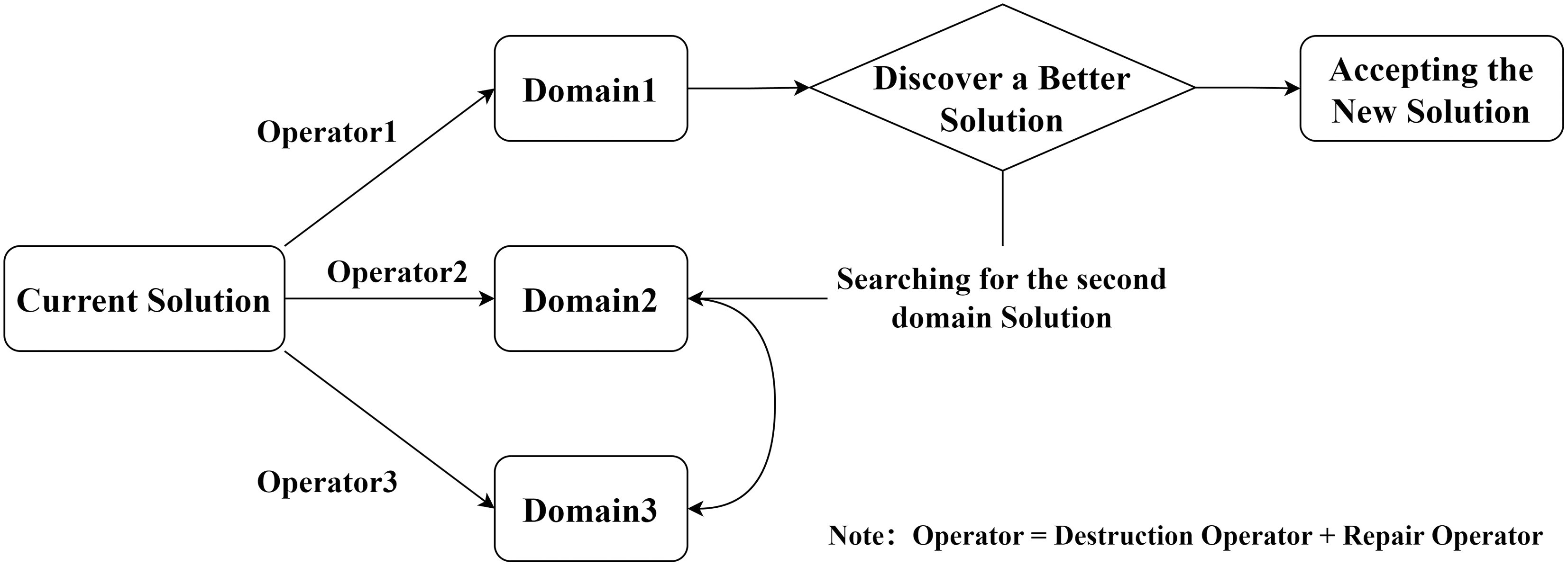
Figure 1.
Flowchart of the ALNS algorithm.
The operator functions of the model described in this article encompass the skip-stop operator and the termination operator, serving as the execution functions for the destruction operator and the repair operator, respectively.
Skip-stop operator
-
During the process of skip-stopping, the number of executions of the skip-stop operator γ1 is determined by the minimum number of skip-stops and the minimum service frequency. The γ1 expression is as follows:
$ {\gamma }_{1}=(1-\sigma ) \cdot \left(\sum\nolimits_{k=1}^{K}\sum\nolimits_{i=1}^{S}x_{i}^{k}-num_{k}^{lb} \cdot {f}_{i}\right) $ (51) Overall upward rounding (numklb represents the minimum number of skip-stops for the k-th train, fi represents the minimum number of stops at the i-th station, initialized as 3 before), where σ is a random number between 0 and 1.
(1) Skip-Stop Operator 1 (Random Skip-Stop): randomly select a vehicle k from (1, k), and then randomly set skip-stops. For i
$\in $ 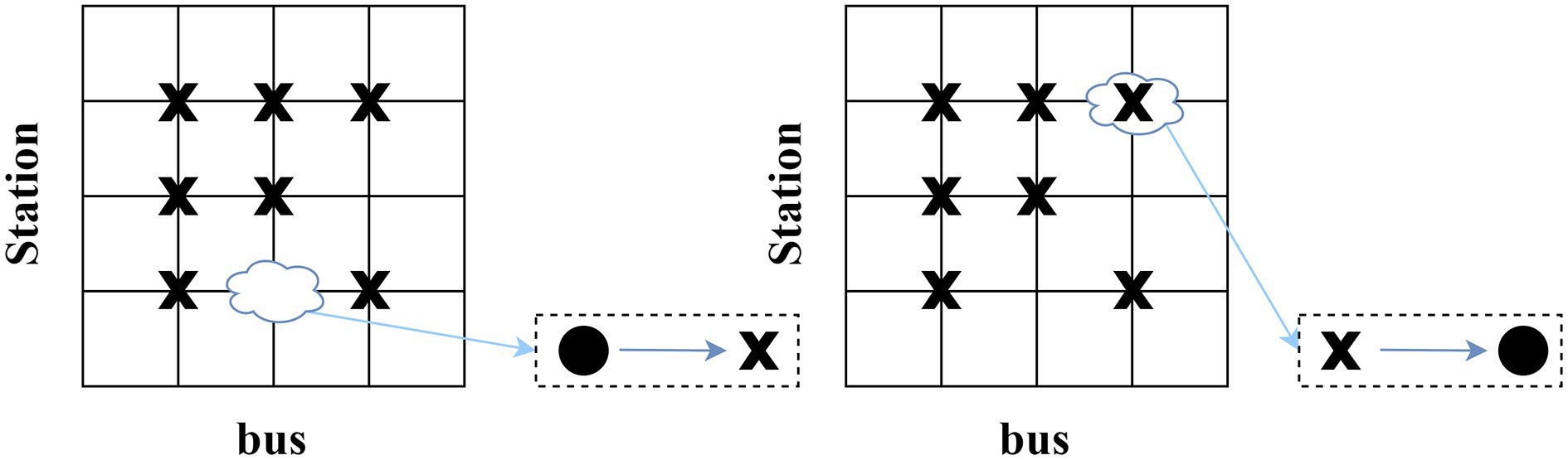
Figure 2.
Randomly skip/stop.
(2) Skip-Stop Operator 2 (Service Frequency Skip-Stop): firstly, search for the station with the highest service frequency, and then let curf = 0, if
$ \sum\nolimits_{{k}=1}^{{K}}\sum\nolimits_{{i}=1}^{{S}}{x}_{{i}}^{{k}}> \text{cu}{\mathrm{r}}_{\mathrm{f}} $ $\in $ $ {x}_{\text{cu}{\mathrm{r}}_{\mathrm{s}-1}}^{{k}}=1 $ $ \sum\nolimits_{\mathrm{i}=1}^{\text{cu}{\mathrm{r}}_{\mathrm{s}-1}}{x}_{{i}}^{{k}}> \text{cu}{\mathrm{r}}_{\text{stop}} $ $ \text{cu}{\mathrm{r}}_{\text{stop}}=\sum\nolimits_{\mathrm{i}=1}^{{S}}{x}_{{i}}^{{k}} $ $ {{\mathrm{cur}}}_{k} $ $ {x}_{\text{cu}{\mathrm{r}}_{\mathrm{s}-1}}^{\text{cu}{\mathrm{r}}_{\mathrm{k}}} $ 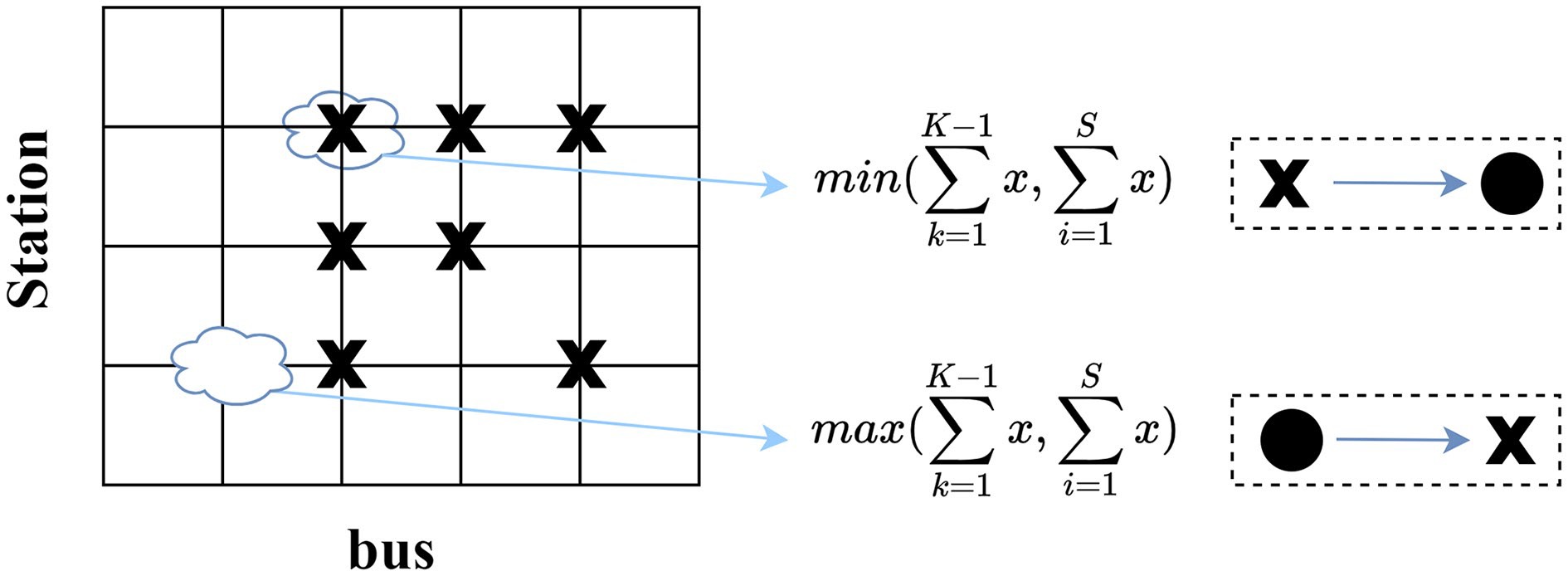
Figure 3.
Frequency_driven skip/stop.
(3) Skip-Stop Operator 3 (Demand Skip-Stop): initialize the demand
$ {{\mathrm{cur}}}_{demand} $ $\in $ $\in $ $ {{\mathrm{cur}}}_{k} $ $ {{\mathrm{cur}}}_{s} $ $ x_{cu{r}_{s-1}}^{cu{r}_{k}} $ 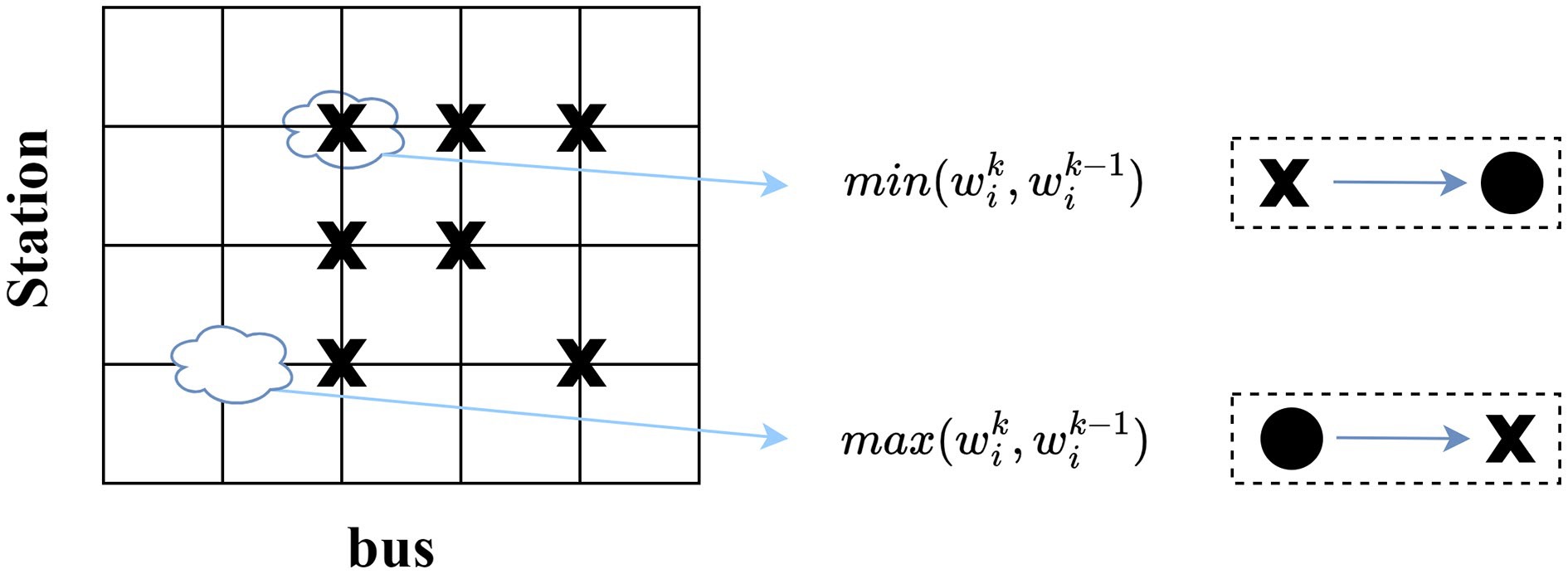
Figure 4.
Demand-driven skip/stop.
-
The number of executions for the termination criterion is γ2, and the expression for γ2 is:
$ {\gamma }_{2}=(1-\sigma ) \cdot ((S \cdot K)-\sum\nolimits_{k=1}^{K}\sum\nolimits_{i=1}^{S}x_{i}^{k}) $ (52) Rounding up the formula, where
$ \sigma $ (1) Termination Criterion 1: randomly select k from (1, K). If
$ \sum\nolimits_{i=1}^{S}\left(1-x_{i-1}^{k}\right)\leq {f}_{i} $ $ x_{i-1}^{k} $ $ \sigma $ $ x_{-i-1}^{k} $ (2) Termination Criterion 2: first, search for the station with the lowest service frequency. Initialize
$ cu{r}_{f} $ $ \sum\nolimits_{k=1}^{K}\sum\nolimits_{i=1}^{S}x_{i}^{k} \lt cu{r}_{f} $ $ cu{r}_{f}=\sum\nolimits_{k=1}^{K}\sum\nolimits_{i=1}^{S}x_{i}^{k} $ $ cu{r}_{s} $ $ cu{r}_{s} $ $ cu{r}_{stop} $ $\in $ $ x_{cu{r}_{s}-1}^{k} $ $ \sum\nolimits_{i=1}^{cu{r}_{s}-1}x_{i}^{k}\leq cu{r}_{stop} $ $ \sum\nolimits_{i=1}^{S}\left(1-x_{i-1}^{k}\right) \gt {f}_{i} $ $ \text{cu}{\mathrm{r}}_{\mathrm{s}}\mathrm{top}=\sum\nolimits_{i=1}^{S}x_{i}^{k} $ $ cu{r}_{k} $ $ x_{\text{cu}{\mathrm{r}}_{\mathrm{s}-1}}^{\text{cu}{\mathrm{r}}_{\mathrm{k}}} $ (3) Termination Criterion 3: let the demand be given, with k
$\in $ $\in $ $ cu{r}_{k} $ $ cu{r}_{s} $ $ x_{cu{r}_{s-1}}^{cu{r}_{k}}=1 $ $ destro{y}_{i}d $ $ destro{y}_{id} $ $ repai{r}_{id} $ $ repai{r}_{id} $ -
In the experiments of this chapter, three bus routes are designed and labeled as 1, 2, and 3, respectively. Route 1 has 10 stops (|S| = 10) with a randomly distributed passenger arrival rate, meaning that the probability of passengers arriving at stop i and then proceeding to a subsequent stop j, where j
$\in $ Parameter settings
-
Based on these settings, this project designed two groups of experiments (as shown in Table 2). The first group varies the number of runs on the three routes, with |K| = 3, 4, 5, and adjusts the average waiting time of passengers accordingly (examples 1−9). All examples in this group are solved using the ALNS algorithm designed in Algorithm and operator introduction. The second group sets |K| = 4 and uses both the Gurobi solver and the ALNS algorithm to solve the problems on the three routes (examples 2, 5, 8, and 10−12). Other input parameters are set as shown in Table 3.
Table 2. Instances of numerical experiments.
No. Number of bus
runs/tripsRoute Average waiting time
for passengers (min)Solution method 1 |K| = 3 1 10 ALNS 2 |K| = 4 1 8 ALNS 3 |K| = 5 1 6 ALNS 4 |K| = 3 2 10 ALNS 5 |K| = 4 2 8 ALNS 6 |K| = 5 2 6 ALNS 7 |K| = 3 3 10 ALNS 8 |K| = 4 3 8 ALNS 9 |K| = 5 3 6 ALNS 10 |K| = 4 1 8 Gurobi 11 |K| = 4 2 8 Gurobi 12 |K| = 4 3 8 Gurobi Table 3. Parameters settings in numerical experiments.
Parameter Symbol Value Maximum capacity C 30 Travel time between stops (min) ti 2 Stopping time at stations (min) p Originating station: 5, Intermediate stations: 1, Terminating station: 0 Minimum headway time (min) hmin 4 Maximum headway time (min) hmax 12 Minimum service frequency per stop fmin 1 Time saving weight β1 0.4 Risk weight β2 0.6 Static risk value at stops μ 2 Number of iterations epochs 100 Weight updating step size pu 5 Annealing rate phi 0.9 Numerical experiment results
-
The results of the first group of experiments are shown in Table 4. From the results, it can be seen that compared with passengers arriving randomly (examples 1~3), when the passenger arrival rate follows a normal distribution (examples 4~6), passengers save more time in total, the risk of virus transmission among vehicles is smaller, and the objective function is also smaller. This means that when the passenger arrival rate follows a normal distribution, the effect of skip-stop scheduling is better. Comparing Route 2 (examples 4~6) and Route 3 (examples 7~9), it can be seen that when the bus route is longer and there are more stops along the route, increasing the number of bus runs can significantly reduce the number of stranded passengers. The results of the second group of experiments are shown in Table 5. When the number of stops is 10 and 20, ALNS can obtain a good solution within 20 s. When the number of stops is 20, it takes 146 min for the Gurobi solver to obtain the optimal solution, which means that although the model can be approximately represented in a linear form when considering passenger stranding, the solution time is too long for large-scale scheduling problems. The results in Table 5 demonstrate the efficiency and superiority of the ALNS algorithm.
Table 4. Results of the first set of numerical experiments.
No. Time saved (min) Risk of transmission Objective function Maximum consecutive skipped stops (stations) Maximum no. of stranded passengers (persons) 1 −198 7,534 4,441.2 4 10 2 70 9,813 5,915.8 4 4 3 −163 15,813 9,422.6 5 19 4 45 5,557 3,352.2 4 11 5 −122 6,567 3,891.4 5 8 6 −106 6,910 4,103.6 5 10 7 −3,648 53,471 30,623.4 8 44 8 −1,648 73,253 43,292.6 7 34 9 −1,791 89,457 52,957.8 9 23 Table 5. Results of the second set of numerical experiments.
No. Objective function Running time (s) 2 5,915.8 7.22 10 5,833.4 478.6 5 3,891.4 7.5 11 3,376.3 512.3 8 43,292.6 18.15 12 42,726.9 8,756 -
As a real-case example, the bus route selected in this article is Route 1 in Changde City (as shown in Fig. 5), Hunan Province. This route operates in the Wuling District of Changde City and is a downtown line with a total length of approximately 11 km. This article selects the upstream route, starting from the Agricultural Market Station and ending at the Hunan Vocational College of Education Station. In between, it passes through densely populated areas such as the First People's Hospital of Changde, Changde Vocational and Technical College, and Changde Vocational and Technical College of Finance and Economics. Therefore, the study of bus skip-stop scheduling considering the risk of infection in this article has strong practical significance.
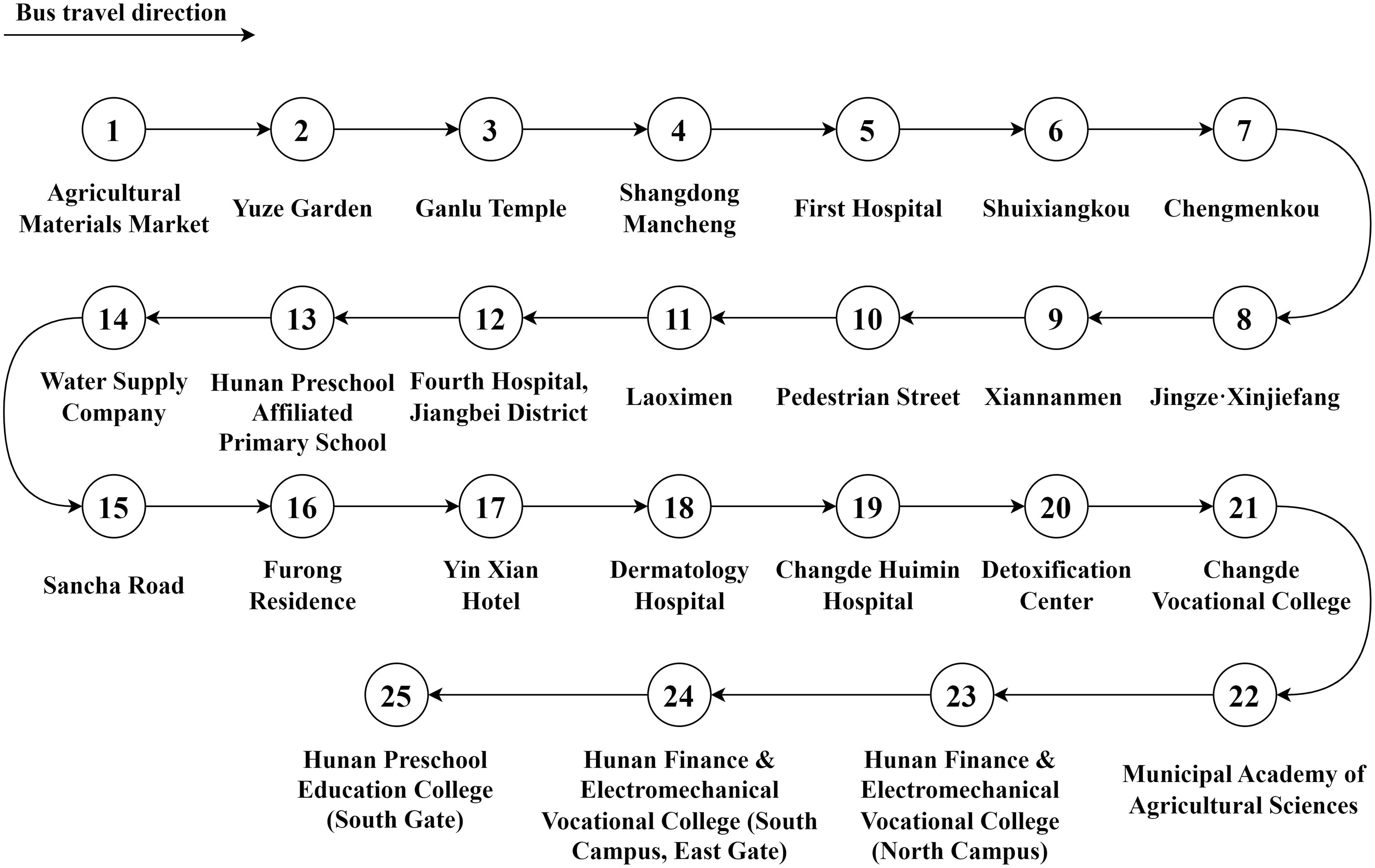
Figure 5.
Changde No.1 bus route map.
There are 25 bus stops along the route (as shown in Fig. 2), numbered 1−25 (S = {1, 2, ..., 25}) in the direction of travel. The time range considered is from 13:00 to 16:00 in the afternoon, involving 25 upstream bus services. The dynamic passenger flow demand used in the experiment is passenger swiping data collected by the bus IC card swiping system on October 7, 2022. For simplicity, this article only considers the issue of passenger stranding without considering passenger transfers.
Passenger OD matrix construction
-
Since the bus IC card system only records the boarding time and boarding stop of passengers, we infer the missing alighting stops using a statistical estimation approach. Based on historical operational data, passengers in the study area travel an average of approximately four stops; thus, we assume that the travel distance follows a normal distribution. For a passenger boarding at stop i, the probability of alighting at stop j is given by:
$ p(j)=\dfrac{1}{\sqrt{2\pi}}\cdot exp\left(-\dfrac{\left(j-\mu\right)^2}{2\delta^2}\right) $ (53) where, μ is the mean travel distance, and δ is the standard deviation. Based on the boarding volume bik, the estimated number of passengers alighting at stop j is:
$ t(j)=b_i^k\cdot p(j) $ (54) This allows us to construct the origin–destination (OD) matrix, as shown in Table 6, and compute the arrival rate λij between stops i and j.
It should be noted that assuming a normal distribution for passenger travel distances is a commonly used method for OD inference when alighting information is unavailable[55]. Nevertheless, this assumption may not fully capture actual travel patterns: it may overestimate long-distance OD if most passengers travel short distances, or underestimate long-distance OD if long-distance commuters are prevalent. Such deviations may introduce some bias into the estimation of onboard loads, exposure risk, and skip-stop scheduling results, although the approach remains a widely accepted and practical solution under data limitations.
Table 6. Passenger OD matrix during the research period.
Off \on 1 2 3 4 5 6 7 8 9 10 11 12 13 14 15 16 17 18 19 20 21 22 23 24 1 − − − − − − − − − − − − − − − − − − − − − − − − 2 4 − − − − − − − − − − − − − − − − − − − − − − − 3 10 0 − − − − − − − − − − − − − − − − − − − − − − 4 20 2 2 − − − − − − − − − − − − − − − − − − − − − 5 26 4 6 3 − − − − − − − − − − − − − − − − − − − − 6 20 5 11 6 6 − − − − − − − − − − − − − − − − − − − 7 10 4 14 12 15 2 − − − − − − − − − − − − − − − − − − 8 4 2 11 15 29 5 2 − − − − − − − − − − − − − − − − − 9 1 0 6 12 36 11 4 1 − − − − − − − − − − − − − − − − 10 0 0 2 6 29 14 7 3 4 − − − − − − − − − − − − − − − 11 0 0 0 3 15 11 9 5 8 3 − − − − − − − − − − − − − − 12 0 0 0 0 5 5 7 6 16 7 2 − − − − − − − − − − − − − 13 0 0 0 0 0 2 4 5 20 14 4 5 − − − − − − − − − − − − 14 0 0 0 0 0 0 2 3 16 17 8 11 1 − − − − − − − − − − − 15 0 0 0 0 0 0 0 0 8 14 11 22 1 1 − − − − − − − − − − 16 0 0 0 0 0 0 0 0 3 7 8 27 2 3 1 − − − − − − − − − 17 0 0 0 0 0 0 0 0 1 2 4 22 4 7 2 0 − − − − − − − − 18 0 0 0 0 0 0 0 0 0 0 2 11 2 9 4 2 0 − − − − − − − 19 0 0 0 0 0 0 0 0 0 0 0 4 1 7 5 3 0 0 − − − − − − 20 0 0 0 0 0 0 0 0 0 0 0 0 0 3 4 4 0 0 0 − − − − − 21 0 0 0 0 0 0 0 0 0 0 0 0 0 1 2 3 1 0 0 0 − − − − 22 0 0 0 0 0 0 0 0 0 0 0 0 0 0 0 2 0 2 1 1 1 − − − 23 0 0 0 0 0 0 0 0 0 0 0 0 0 0 0 0 0 0 1 1 3 0 − − 24 0 0 0 0 0 0 0 0 0 0 0 0 0 0 0 0 0 0 1 2 6 0 0 − 25 0 0 0 0 0 0 0 0 0 0 0 0 0 0 0 0 0 0 0 2 16 0 0 0 Station risk assessment
-
To obtain the static risk value for each stop, we consider the attractiveness of the stop itself and the surrounding land use planning for evaluation.
Determining the inherent risk value of the stop
-
The stop attractiveness rate reflects the inherent risk value of the stop. The higher the number of passengers boarding at a stop, the greater the attractiveness intensity, and accordingly, the greater the risk of passengers boarding at that stop being infected. According to Dai & Chen[56], there is symmetry in the passenger flow between the upstream and downstream directions, meaning that the ratio of the number of passengers boarding at each upstream stop to the total number of passengers boarding is similar to the ratio of the number of passengers getting off at the corresponding downstream stop to the total number of passengers getting off. Therefore, we choose the number of passengers boarding at downstream stops to determine the inherent risk value of the stop.
$ {X}_{i}=\dfrac{b_{i}^{'}}{\displaystyle\sum\nolimits_{i=1}^{|S|}b_{i}^{'}} $ (55) where, Xi represents the attractiveness intensity of stop i, and b'i represents the number of passengers boarding at the corresponding stop i in the opposite direction.
Assessment of the surrounding risk at stations
-
When there are densely populated places such as shopping malls, hospitals, schools, etc., around the station, the risk value of the station will also increase. Therefore, we also consider the surrounding land planning when assessing the risk of the station. The distance between bus stops is generally between 500 and 600 m, and we take half of the upper limit, which is 300 m, as the calculation basis. Based on the land use planning within 300 m of each station and the static risk values of different land types, we assess the surrounding risk value of each station:
$ G_{i}^{*}=\sum {L}_{im}{\alpha }_{im} $ (56) where, G*i represents the risk value around the station, which needs to be normalized to obtain Gi. Lim represents the floor area of the k-th type of land use within 300 m of stop i. αim represents the static risk value per unit area of the k-th type of land use within 300 m of stop i. By combining the risk value of the station itself and the risk value around the station, the static risk value of the station is calculated:
$ {\mu }_{i}=\dfrac{{\beta }_{1}{X}_{i}+{\beta }_{2}{G}_{i}}{\displaystyle\sum\nolimits_{j=1}^{|S|}{\beta }_{1}{X}_{j}+{\beta }_{2}{G}_{j}} $ (57) where, β1 represents the weight of the risk value of the station itself, and β2 represents the weight of the risk value around the station. β1 + β2 = 1, and β1 + β2 = 0.5. The calculated static risk value of the station is shown in Table 7.
Table 7. Static risk value of the site.
Station number Static risk value Station number Static risk value 1 18 14 3 2 3 15 1 3 4 16 6 4 4 17 1 5 11 18 1 6 0 19 5 7 1 20 0 8 1 21 8 9 1 22 0 10 0 23 5 11 10 24 9 12 3 25 5 13 1 Capacity and headway considerations
-
The passenger capacity of urban public transportation is generally around 40 people. During the epidemic period, many regions issued regulations to limit the passenger capacity of public transportation. For example, Harbin required that the number of passengers be limited to 50% of the passenger capacity, and Tianjin set 60% as the red line for bus passenger capacity. As the epidemic situation improves, the corresponding regulations have also been relaxed. In this study, we set the maximum capacity at 75% of the passenger capacity, or 30 people. Some studies suggest that there is a relationship between the average waiting time of passengers and the departure interval W = 2.34 + 0.26
$\mu $ $\mu $ Table 8. Solving parameters.
Parameter Symbol Value Number of buses/shift |K| 25 Number of stops |S| 25 Maximum capacity C 30 Travel time between stops (min) ti 2 Stopping time at stations (min) p Originating station: 5, Intermediate stations: 1, Terminating station: 0 Average waiting time of passengers per minute β 4.4 Minimum headway time (min) hmin 4 Maximum headway time (min) hmax 12 Minimum service frequency per stop fmin 1 Time saving weight β1 0.4 Risk weight β2 0.6 Number of iterations epochs 100 Weight updating step size pu 5 Annealing rate phi 0.9 Results and analysis
-
We used the ALNS method introduced in the fourth part to solve the integer programming model constructed in the third part. Based on the above original data, we obtained an optimal skip-stop scheduling strategy, where the service status of buses at each station and the number of passengers boarding and disembarking at that station are shown in Fig. 6.
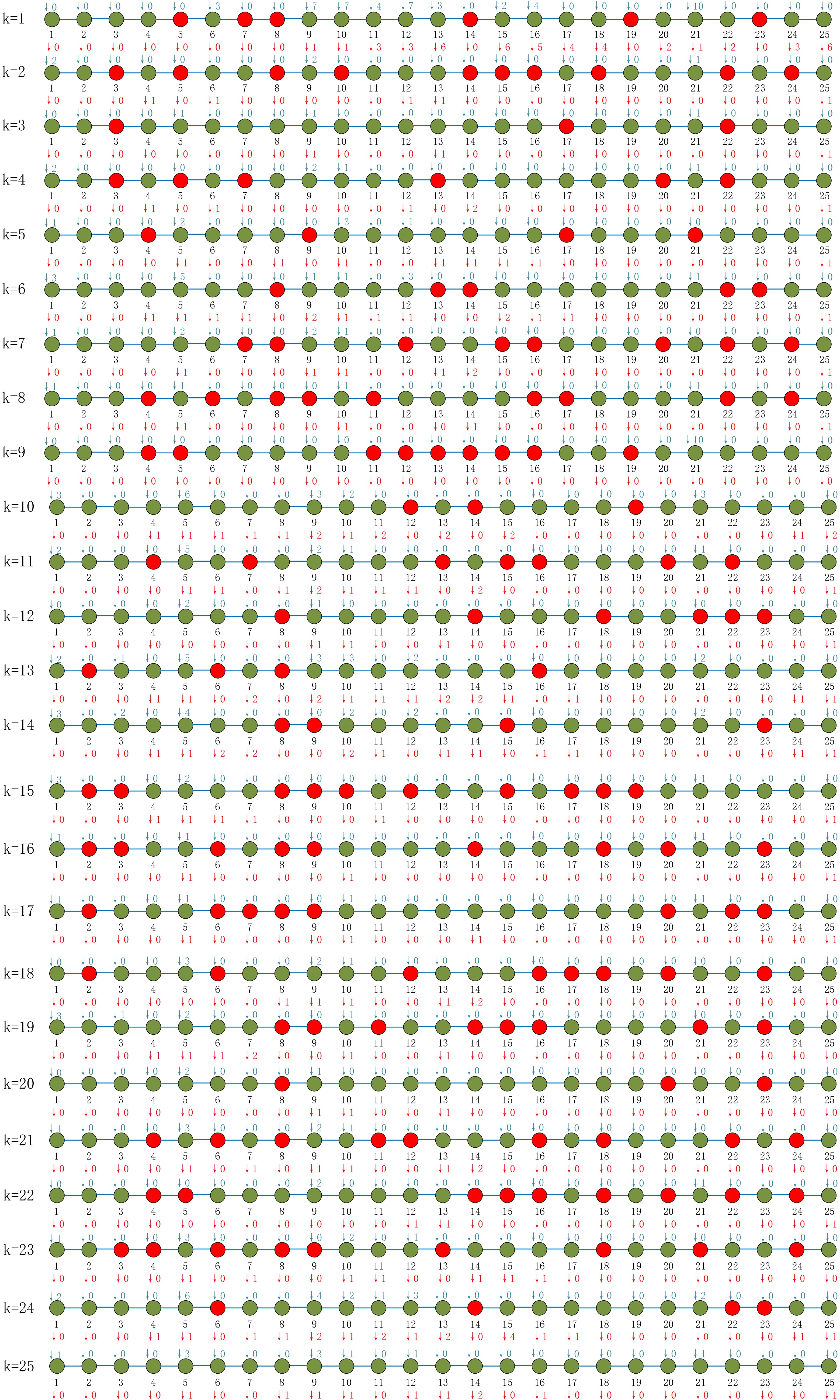
Figure 6.
Original scheduling skip station plan: Red stations indicate skipped stops, while green stations indicate stops. The upper number represents the number of boarding passengers, and the lower number represents the number of alighting passengers. In the first half of the route (stations 1–13), where passenger flow is relatively concentrated, buses stop more frequently.
Compared with the stop-at-every-station strategy, the skip-stop scheduling strategy reduces the total passenger travel and waiting time by 197 min, based on the calculations in Table 9.
Table 9. Original scheduling solution results.
Saved time Risk value Objective function 197 298,479 179,166.2 From the original case, we observed that some trains (e.g., k = 2) carried very few passengers, indicating that fewer trains are required under the skip-stop strategy compared to the stop-at-every-station service. Accordingly, we reduced the number of trains to 12 and recalculated the average passenger waiting time as 8 min. Based on these adjustments, we re-solved the model and obtained the optimal skip-stop scheduling strategy shown in Fig. 7. Skipped stations are relatively evenly distributed along the route. In the upper section with high passenger flow, the strategy typically alternates between stopping and skipping stations to shorten travel time while mitigating cumulative in-vehicle exposure risk. In the lower section with lower passenger flow, consecutive skipping is frequently applied, which also reduces travel time.
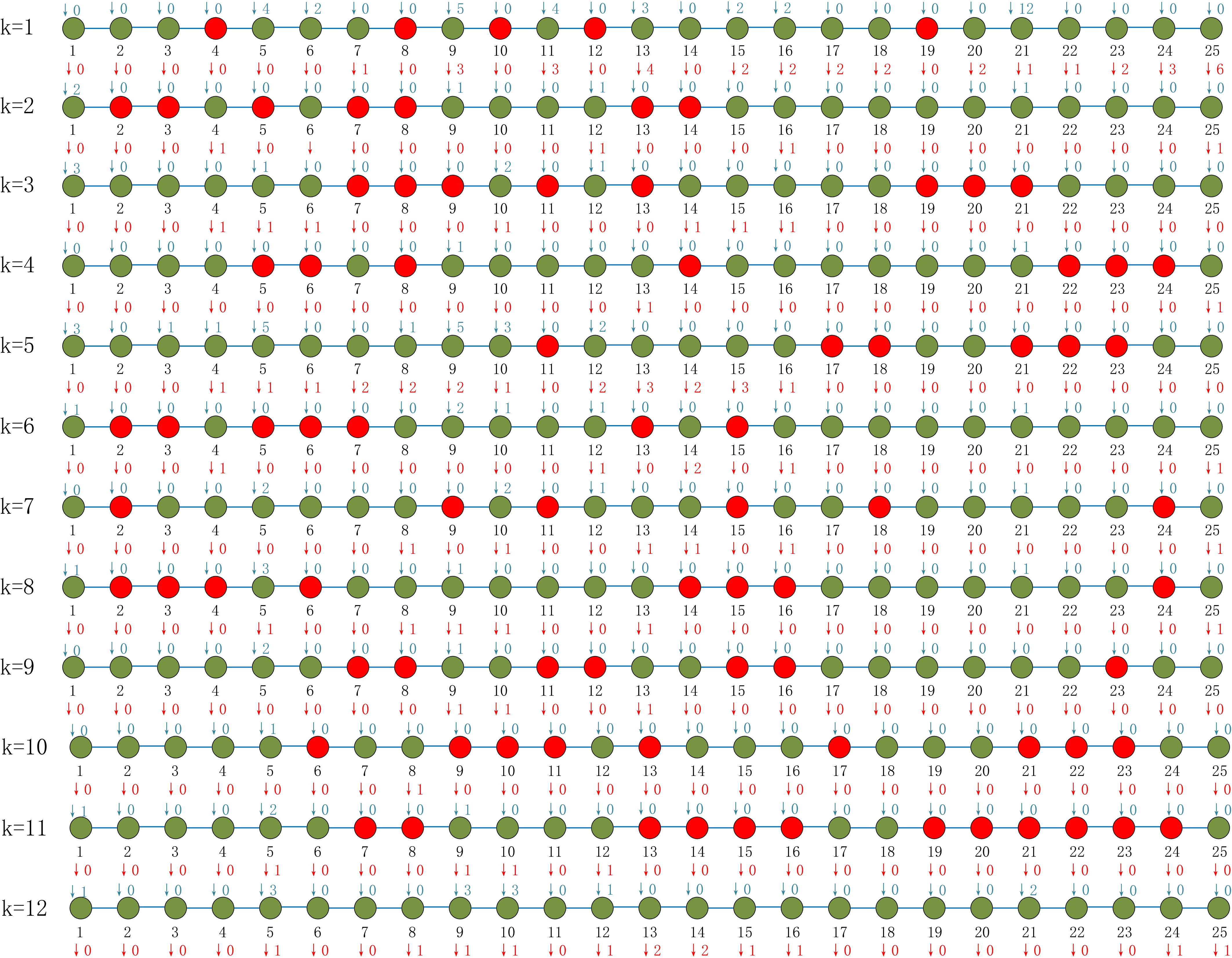
Figure 7.
Optimal skip-stop scheduling with reduced train frequency: Red and green markers indicate skipped and served stations, respectively, with each station labeled by the number of boarding and alighting passengers. The skip-stop pattern adapts to passenger flow: 'stop once, skip once' in high-flow upper sections and consecutive skipping in low-flow lower sections, with skipped stations evenly distributed along the route.
Compared with the stop-at-every-station service model, the reduced-frequency skip-stop scheduling saves 86 min in total passenger travel time. Compared with the original case, the risk value of the reduced-frequency skip-stop strategy is reduced by 58.8%, demonstrating its effectiveness in mitigating infection risk while maintaining service efficiency based on the calculations in Table 10.
Table 10. Scheduling solution results for reducing shifts.
Saved time Risk value Objective function 86 122,919 73,785.8 In the objective function of the model, both the total waiting time related to service quality and the passenger flow aggregation risk related to operation safety are considered. In the objective, the trade-off between the two goals needs to be balanced through weight coefficients. This article tested six different values for the trade-off coefficient, with β1 taking values of 0, 0.2, 0.4, 0.6, 0.8, and 1.0, respectively. The corresponding calculation results for each value are shown in Table 11.
Table 11. Weighing coefficient value.
$ {\beta }_{1} $/$ {\beta }_{2} $ Saved time Risk value Objective function 0/1 13 10,916 6,554.8 0.2/0.8 59 119,393 103,536.4 0.4/0.6 86 122,919 73,785.8 0.6/0.4 99 120,412 56,224.2 0.8/0.2 97 121,659 20,409.4 1/0 110 148,444 110 It can be seen that as β1 increases, the savings in passenger waiting time show an upward trend, while the corresponding risk value increases. By setting different weight coefficients, a reasonable trade-off can be made between safety and service quality, which is more meaningful for actual operations.
Importantly, the results reveal two key correlations that explain the reduction in infection risk after decreasing train frequency:
(1) Passenger flow–infection risk correlation: Stations with higher passenger flow contribute more to cumulative in-vehicle exposure. By reducing stops at low-demand stations or decreasing train frequency, the total number of passengers on board simultaneously is reduced, directly lowering infection risk.
(2) Skip-stop frequency–travel time correlation: Alternating stop-skip patterns in high-flow areas maintain service efficiency, keeping average travel time low, while consecutive skipping in low-flow areas further reduces unnecessary dwell time. Together, these mechanisms explain why fewer trains under the optimized skip-stop plan can simultaneously reduce total travel time and in-vehicle infection risk.
-
Ensuring travel demand through public transportation while meeting epidemic prevention requirements remains a critical challenge during sudden public health events such as the COVID-19 pandemic. This study proposes a risk-aware circular skip-stop bus scheduling model that jointly optimizes passenger travel time and cumulative in-vehicle infection risk. A mixed-integer programming formulation is developed to determine station-level skip-stop strategies, and an Adaptive Large Neighborhood Search (ALNS) algorithm is designed to efficiently generate high-quality solutions for this multi-objective, multi-constraint combinatorial problem.
The ALNS algorithm demonstrates strong adaptability and scalability. Its main innovations include an adaptive operator weight update mechanism, customized destruction and repair operators incorporating skip-stop and stop-protection rules, and a simulated annealing-based probabilistic acceptance criterion for non-monotonic multi-objective exploration. The algorithm achieves outstanding large-scale performance, obtaining high-quality solutions within 20 s for a 25-station, 25-trip real-world route, whereas an exact solver requires 146 min. These features allow ALNS to efficiently explore large neighborhoods, accommodate multiple custom operators, and scale to large instances, making it highly compatible with the proposed model and practically effective.
Although immediate societal focus on COVID-19 has waned, the proposed modeling framework remains broadly relevant. Beyond COVID-19, it can be applied to other major respiratory and airborne diseases, such as seasonal influenza, RSV, and mycoplasma pneumonia. By integrating minimization of passenger contact time with cumulative infection risk assessment, the model provides actionable decision support for routine bus operations and public health emergency scheduling. Numerical results indicate that the optimized skip-stop strategy effectively reduces in-vehicle infection risk, enhances operational safety, and achieves a modest reduction in total travel time. Transit operators can flexibly adjust the relative weights of travel time and infection risk based on epidemic severity and passenger flow, improving the model's operational relevance. Future research could extend the model to network-level analysis and incorporate stochastic passenger demand to develop robust skip-stop scheduling strategies under uncertainty.
-
The authors confirm their contributions to the paper as follows: study conception and design: Sun P, Xiao L, Vasilina G; data collection: Zhong L, Vasilina G, Wang L; analysis and interpretation of results: Sun P, Zhong L, Wang L; draft manuscript preparation: Sun P, Zhong L, Wang L, Xiao L. All authors reviewed the results and approved the final version of the manuscript.
-
The datasets generated during and/or analyzed during the current study are are available from the corresponding author on reasonable request.
-
All the authors thank the financial support from the National Natural Science Foundation of China (Grant No. 72132007) and the Key Program of the National Natural Science Foundation of China (Grant No. 72431006), the Humanities and Social Sciences Foundation of the Ministry of Education of China (Grant No. 24YJC630095), and the project supported by CACMS (TJU) (Grant No. FM-ZX-2025-TJ02-003).
-
The authors declare that they have no conflict of interest.
- Copyright: © 2026 by the author(s). Published by Maximum Academic Press, Fayetteville, GA. This article is an open access article distributed under Creative Commons Attribution License (CC BY 4.0), visit https://creativecommons.org/licenses/by/4.0/.
-
About this article
Cite this article
Zhong L, Sun P, Vasilina G, Wang L, Xiao L. 2026. Bus station-skip scheduling problem with passenger infection risk. Digital Transportation and Safety 5(2): 84−97 doi: 10.48130/dts-0026-0007 

Bus station-skip scheduling problem with passenger infection risk
- Received: 10 December 2025
- Revised: 14 January 2026
- Accepted: 20 March 2026
- Published online: 29 June 2026
Abstract: The present research offers optimized strategies for bus scheduling that take into account the risk perceptions of infectious diseases in the post-pandemic era. These strategies aim to rebuild public trust in transportation systems and provide solutions for buses to mitigate risks associated with seasonal infectious diseases, such as influenza and respiratory infections. We address the risk of disease transmission by developing a precise mixed-integer programming model that optimizes stop-hopping strategies from a system-wide perspective, focusing on minimizing passenger infection risk and reducing overall travel time at each stop. To enhance the model's accuracy, we leverage advancements in smart bus technology, enabled by the Internet of Things and other innovations. By analyzing bus route data from Changde City, Hunan Province, we independently design an adaptive large neighborhood search (ALNS) algorithm. This algorithm produces a high-quality stop-hopping scheduling strategy with greater speed and accuracy than traditional methods. The results demonstrate that the optimized strategy significantly reduces virus transmission risk, shortens total passenger travel time, and enhances operational safety.