High-throughput phenotyping tools for blueberry count, weight, and size estimation based on modified YOLOv5s

Blueberry is known for its high levels of antioxidants and other health-promoting compounds, including fiber, vitamins, and manganese^[1,2]. Driven by consumers' desires for healthy food, global blueberry production has more than doubled between 2010 and 2019 from 439,000 to nearly 1.0 million metric tons^[3]. As the No. 1 blueberry producer in the world, the US generated a total value of USD${\$}$1 billion of blueberries in 2021^[3] and the expansion of the US blueberry market is expected to continue in the coming years^[4]. There are five major types of blueberries produced in various parts of the world. The most common ecotype is highbush blueberry, which can be further divided into northern highbush (Vaccinium corymbosum L.) and southern highbush (V. corymbosom L. interspecific hybrids) depending on chilling requirements^[5]. Rabbiteye blueberry (V. virgatum Ait.) is a native species in the southeastern US that is commonly grown on small-scale farms for U-pick and retail production. Lowbush blueberry (V. angustifolium Ait.) is considered a wild type and is mainly produced in Canada and the Northeastern US primarily for the processed market. Additionally, half-high blueberries are the hybrids of highbush × lowbush primarily produced in the Midwest US for their cold hardiness.

The profitability of the blueberry industry relies on continuous progress in breeding to provide growers with optimal cultivars. However, labor-intensive phenotyping for many blueberry traits has become a major bottleneck for efficient blueberry improvement. Blueberries are routinely evaluated for yield, average berry size, average berry weight, texture, taste, and many other pre- and post-harvest traits for breeding and research purposes. Towards the end of a growing season, blueberries are harvested and brought back to the lab for phenotyping (Fig. 1a). Yield is measured by weighing all the harvested berries for each plant (Fig. 1b). After that, a subset of harvested berries is counted and weighed to calculated average berry weight (Fig. 1c). Berry size is often manually measured with calipers or using machines for fruit firmness and size measurements, such as FruitFirm® 1000 (CVM Inc., Pleasanton, CA, USA) (Fig. 1d, e).

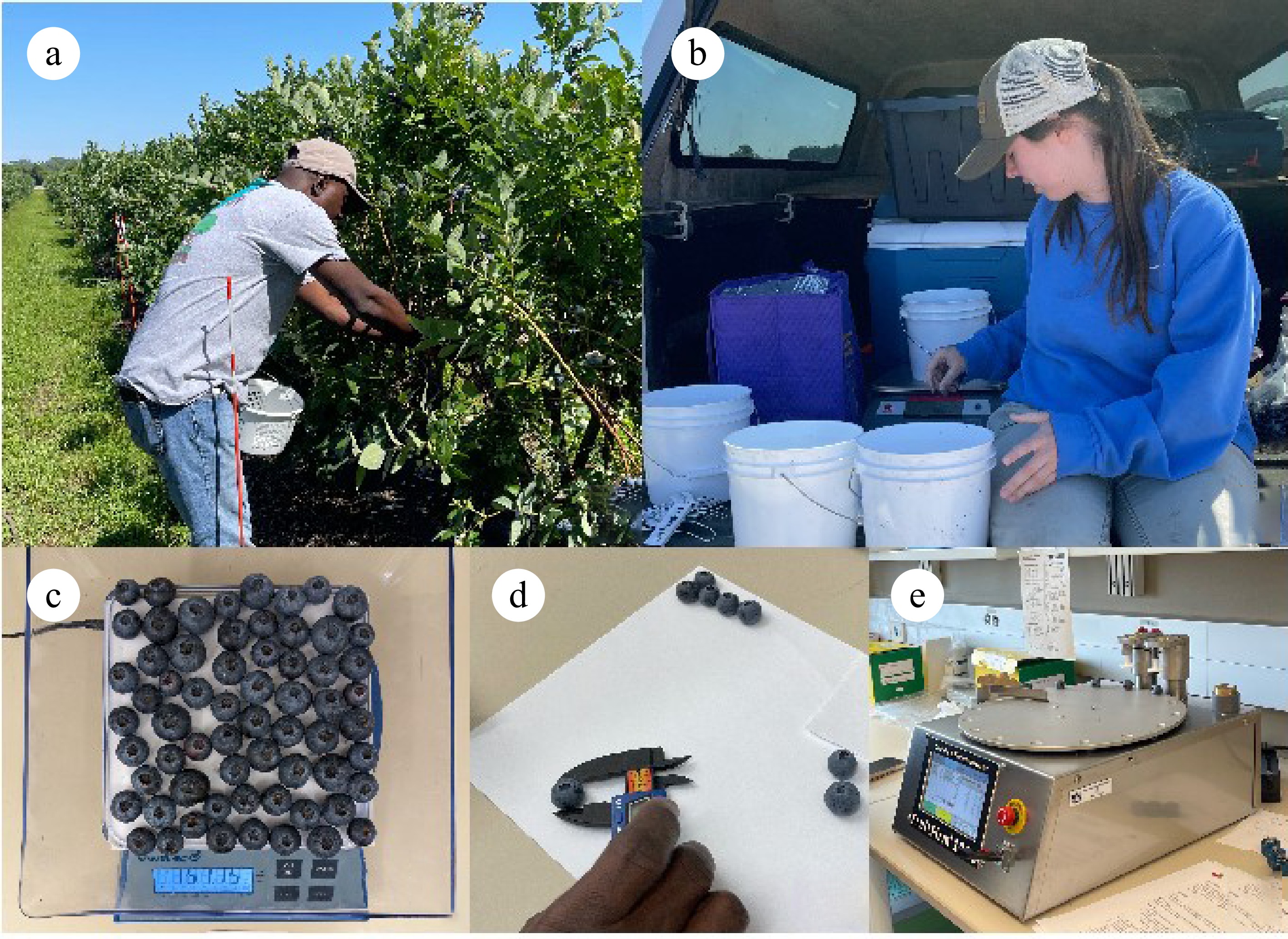
Figure 1. 

Process of blueberry phenotyping for yield, average berry weight, and size. (a) Blueberry harvesting, (b) yield measurement, (c) average berry weight measurement, (d) manual measurement of berry size with an electronic digital caliper, (e) berry size and firmness measurement with FruitFirm® 1000 (CVM Inc., Pleasanton, CA, USA).

Traditional methods for measuring average berry weight are labor-intensive and error-prone. Additionally, the average berry weight is limited in its ability to show variations in berry weight within a plant. Berry size is even more challenging to phenotype manually due to the small size and large number of berries. Some texture measurement instruments such as FruitFirm 1000 (CVM Inc., Pleasanton, CA, USA) can measure firmness and berry size simultaneously^[6,7]. However, not all researchers or growers have access to such equipment. As berry size and weight are highly correlated in blueberries^[8], a high-throughput phenotyping solution for one trait can directly benefit the other.

RGB image-based analysis has been applied in object detection for many agricultural and horticultural crops such as banana (Musa spp.), cotton (Gossypium spp.), oil-seed camellia (Camellia oleifera), and tomato (Solanum lycopersicum)^[9−12]. Object detection models such as You Only Look Once (YOLO), based on convolutional neural networks (CNNs), have been shown to be powerful for crop detection such as tomato (97% accuracy)^[9], and oil-seed camellia (90% accuracy)^[11]. In banana, the integration of deep learning with histogram equalization and Canny edge detection resulted in an accuracy of 86% for counting banana bunches during the harvesting period^[12].

Several studies have explored the application of image-based analysis for blueberry detection and yield estimation. Swain et al.^[13] developed a pixel color threshold model for yield prediction in wild blueberries (Vaccinium angustifolium Ait.), which achieved an R² of 0.97 for predicted versus measured yield. Both YOLOv3 and YOLOv4 were employed for yield estimation of wild blueberries with an R² value of 0.89 of predicted vs measured yield^[14]. For cultivated blueberries such as southern highbush, a hybrid approach employing neural network models and traditional techniques including histogram-oriented gradients, sliding window, and the K-nearest neighbors classifier, achieved detection rates of 94.8%, 94.6%, and 84.4% for mature, intermediate, and young field-grown blueberry plants, respectively^[15]. Mask R-CNN also demonstrated strong performance for field-grown blueberry detection among four southern highbush cultivars, with R² values ranging from 0.85 to 0.93 for model-detected berry count and measured berry count^[16]. A modified version of YOLOv5, incorporating attention and expansion mechanisms, outperformed the baseline YOLOv5 by achieving a 9% higher mean average precision (mAP) in blueberry ripeness detection^[17]. Although many models have been developed for blueberry detection, the capability of real-time detection and sizing through smartphone applications remains limited, likely due to the complexity and volume of existing models. The goal of this study is to develop a robust and lightweight blueberry detection algorithm and a smartphone application for real-time berry count and size phenotyping in the lab setting. The specific objectives of this study were to: (1) develop image processing pipelines for automatic blueberry count and size estimation in the lab setting; (2) implement and enhance CNN models with reduced parameters for blueberry count and size estimation; and (3) develop a smartphone application to enable efficient berry size and weight phenotyping.

A total of 198 images, along with manually measured count and weight data, were used for training and testing algorithms for blueberry count and size estimation. The first dataset contained 48 images of harvested southern highbush blueberries from 24 six-year-old blueberry plants of 9 advanced selections that have not been released as commercial cultivars. Berries were harvested in May 2022 from a research farm at the Auburn University Gulf Coast Research & Extension Center, Fairhope, Alabama, USA (30°32'44.8692" N, 87°52'51.456" W). The second dataset comprised 52 images of blueberries harvested in June 2022 from nine-year-old rabbiteye blueberry plants of three cultivars 'Premier', 'Powderblue', and 'Alapaha'. Plants were grown on a commercial farm in Auburn, AL, USA. The third dataset included 98 images of blueberries harvested from two-year-old plants in May 2023. Twenty-six unique genotypes including six commercial cultivars (one northern highbush cultivar 'Blue Ribbon', two rabbiteye cultivars 'Krewer' and 'Vernon', and three southern highbush cultivars 'Gumbo', 'New Hanover', and 'San Joaquin' and 20 advanced breeding selections (16 southern highbush and four rabbiteye selections) were used in the third dataset. Plants in the third dataset were maintained at the Auburn University E.V. Smith Research Center (Tallasee, AL, 32°29'48.7"N, 85°53'33.8"W) and Brewton Agricultural Research Unit (Brewton, AL, 31°8'38.2" N, 87°2'59.8" W).

Ripe berries were manually harvested and stored at 4 °C for 1−3 d before image and weight data collection. A subset of harvested berries was manually counted and weighed with a VWR® portable balance 1,500 G × 0.05 G (us.vwr.com). Berries were placed with the calyx scar side facing up before weighing. A white printing paper was positioned underneath the transparent weighing boat to enhance the contrast between the berries and the background (Fig. 2). Berry images were captured with a Google Pixel 5A phone clipped onto a SupeDesk® portable cell phone stand (supedesk.com). Total berry weight (g) was recorded, and average berry weight was calculated as total berry weight (g)/berry number. The inside dimension of the weighing boat is 15 cm, which was used as the reference for berry size model calibration. Raw images were manually annotated via the labelImg^[18] tool to identify each berry using a bounding box. This bounding box was created as closely as possible to the outer edge of each berry to accurately measure its true size (Fig. 2c). The histogram in Fig. 2d shows the majority of blueberry sizes in data collection are between 1 and 3 cm².

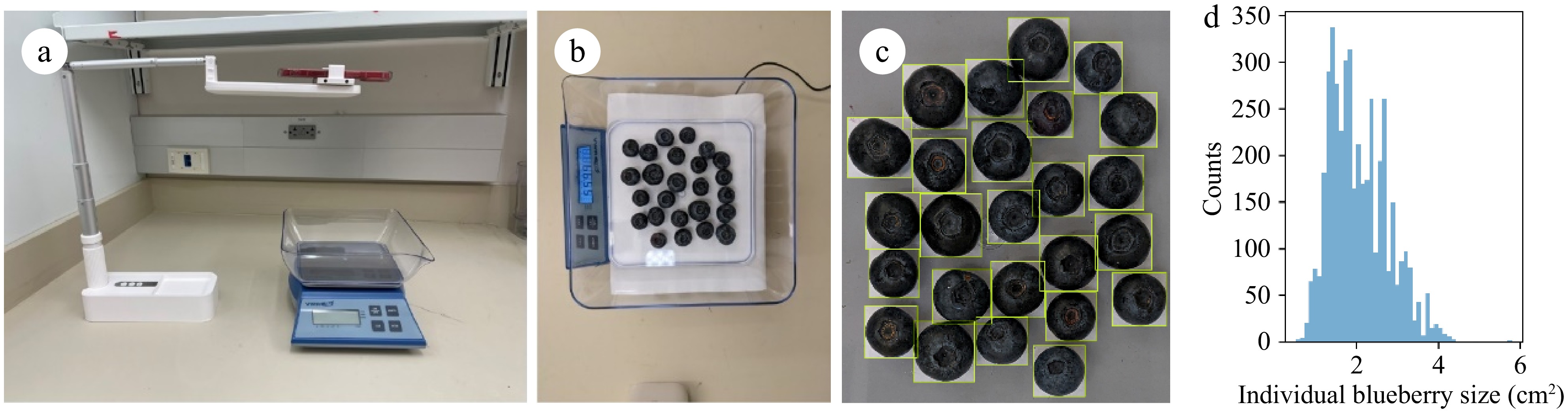
Figure 2. 

Weight data collection: (a) setup of berry weight and image data collection; (b) image of blueberries from one sample; (c) zoomed-in image of manually annotated blueberries; (d) histogram of labeled individual blueberry sizes.

Hough transform based model

Blueberries exhibit a near-round shape, especially when viewed from above. This characteristic has promoted the development of a detection method where individual blueberries could be identified as circular objects. One commonly adopted method to detect circles in an image is the Hough Transform (HT) method. HT is a well-established and traditional technique that can detect patterns of various shapes in an image^[19]. Notably, OpenCV provides an implementation of the Hough Circle method, which is designed for direct detection of circular patterns in a colored image^[20].

In the HT-based method, the initial steps involved resizing the images to one of two resolutions: 2,000 × 1,500 (first and second dataset) or 1,880 × 1,410 pixels (third dataset). The resolution is varied because of variations in photographing distance, this allows the following algorithms to be consistent across datasets without further parameter adjustments. These resized images were then transferred into the Hough Circle Detector, which obtained a set of circles (Fig. 3). The parameters configured for the Hough Circle detector included a 50-pixel minimum distance between the centers and a radius spanning from 25 to 55 pixels. The following blueberry filter was applied to separate the list of circles into two categories: true blueberries and non-blueberries. This filter operated based on the average RGB color and location to identify the outliers (classified as non-blueberries). The average RGB color was computed and analyzed by determining the average of the red (R), green (G), and blue (B) colors within each circle identified by HT. The circle's location was defined by its center. The mean and standard deviation vectors μ and σ were calculated for the five categories [x, y, B, G, R]. Only berries that met the condition [3, 3, n, n, n] × σ ≥ ([x, y, B, G, R] − μ) were classified as true blueberries for the counting process. With n = 2.5 if σ > 100 or else n = 1. The varying average color threshold (n) provides a stronger limit against non-blueberries in images that have a lower blueberry count (Supplementary Fig. S1).

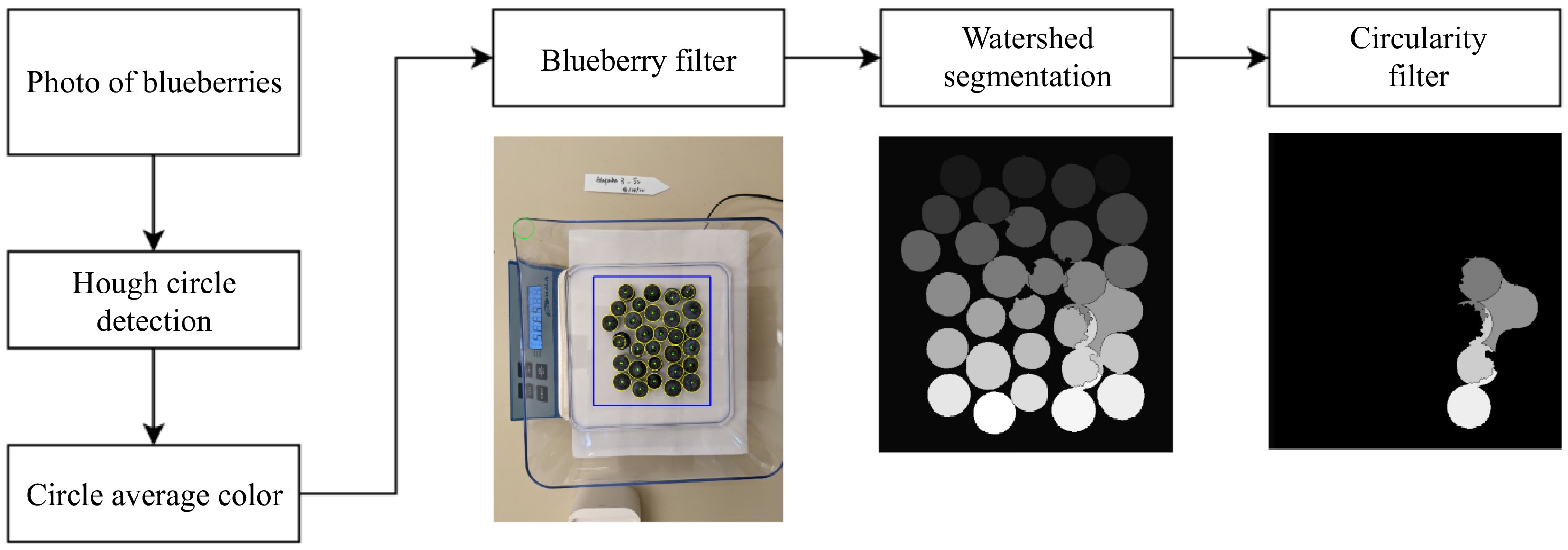
Figure 3. 

Overview of the Hough Transform-based pipeline. After computing the average color of each Hough circle, the blueberry filter determines the count of blueberries (yellow circles) and their segmentation based on Watershed algorithms (middle). The right image shows the blueberries removed in average size estimation based on their segmentation circularity (not removed in counting).

The filtered circle region was marked using three distinct labels: 'individual blueberries', 'undetermined', and 'background', in the processing of subsequent watershed segmentation procedures, implemented by OpenCV^[20]. Each detected blueberry was identified with a blueberry marker, represented by a circle of a constant 25-pixel radius centered on the fruit. The uncertain or indistinct regions were assigned by the undetermined markers with a radius from 26 to 65 pixels while all other areas were designated as the background.

To address the challenges arising from variations in blueberry placement and light conditions, the watershed may mislabel the background between blueberries, as shown in Fig. 3. In response, a supplementary filter based on circularity was applied to eliminate mislabeled objects. The circularity filter assesses the circular nature of each blueberry segmentation by comparing the two key ratios: radius ratio ${R}_{radius}$ and overlap area ratio ${R}_{overlap}$ for each blueberry segmentation region noted as $C$. In Eqn (1), a circle $c$ is defined using the radius $r$ and average location ${\mu }_{C}$ (center $O$) derived from $C$. In Eqn (2), ${R}_{overlap}$ is computed using the overlapping regions of $C$ and circle $c$ placed at $O$, and ${R}_{radius}$ is defined by the ratio of radius $r$ and radius ${r}_{mEnc}$ from the minimum enclosing circle of $C$. Equation (3) applies the threshold to filter for the circular regions (Fig. 3) used to determine the regions used in the weight estimation later.

Data augmentation for deep learning models

The image dataset was shuffled and randomly divided into three subsets with a 70:15:15 ratio, resulting in 3,145, 903, and 875 labeled blueberries, respectively. A series of further augmentations involving orientation changes (± 90°, 180°), lighting changes (± 25% hue, saturation, and ± 10% brightness, exposure), and blur effects (up to 1.5 pixels) were applied to increase the variation of the training dataset, which led to a final training set of 444 images with 9,690 berries (Supplementary Fig. S2).

YOLOv5 based model

YOLOv5 is a popular object detection model for its advantages in speed, accuracy, and robustness of training and deployment on embedded devices^[21]. The YOLOv5 includes five distinct versions: YOLOv5n, YOLOv5s, YOLOv5m, YOLOv5l, and YOLOv5x, which were only different on the depth_multiple and width_multiple applied in the model^[21]. The YOLOv5 is composed of a backbone network, a neck network, and a head network. The backbone network typically employs a deep convolutional neural network: CSPDarknet53, which is responsible for feature extraction from the input images (e.g., blueberry images in this study). The neck network was adapted to the Path Aggregation Networks (PANet) responsible for aggregating image features from multiple layers of backbone networks. The head network includes three detection heads into one anchor-free detection head to provide the prediction function of the bounding boxes, class probabilities, and object confidences.

Modification in the key modules

In this original architecture of YOLOv5 (Fig. 4a), the backbone feature extraction network of YOLOv5 adopts a C3 (Fig. 4b) structure, which results in a large number of parameters, slow detection speed, and limited application. This makes it challenging to apply in certain real-world scenarios such as mobile or embedded devices due to the large and complex model size. The model's size may be too large for the smartphone application and its computational environment (e.g., the Pixel 7 with a Tensor G2 chip and 8GB RAM), potentially causing memory limitations. Also, these scenarios require low latency and fast response times, which is difficult to achieve with such a large and complex model. Hence, we replaced the key modules of C3 in YOLOv5 with the introduction of GhostNet^[22]. GhostNet (Fig. 4c) offers a compelling solution to object detection challenges by prioritizing efficiency without compromising accuracy. The architecture for GhostNet model includes a unique 'ghost' module, incorporating low-rank approximations to significantly reduce the number of parameters and computations. This reduction in computational cost makes GhostNet particularly advantageous for resource-constrained environments and devices with limited processing capabilities, such as edge devices and mobile platforms. Its lightweight design and careful balance between full and 'ghost' convolutional layers contribute to fast inference speeds, ensuring real-time performance in applications like video analysis or image analysis. Overall, GhostNet represents a significant stride in achieving optimal trade-offs between model efficiency and accuracy, catering to the demands of modern object detection tasks.

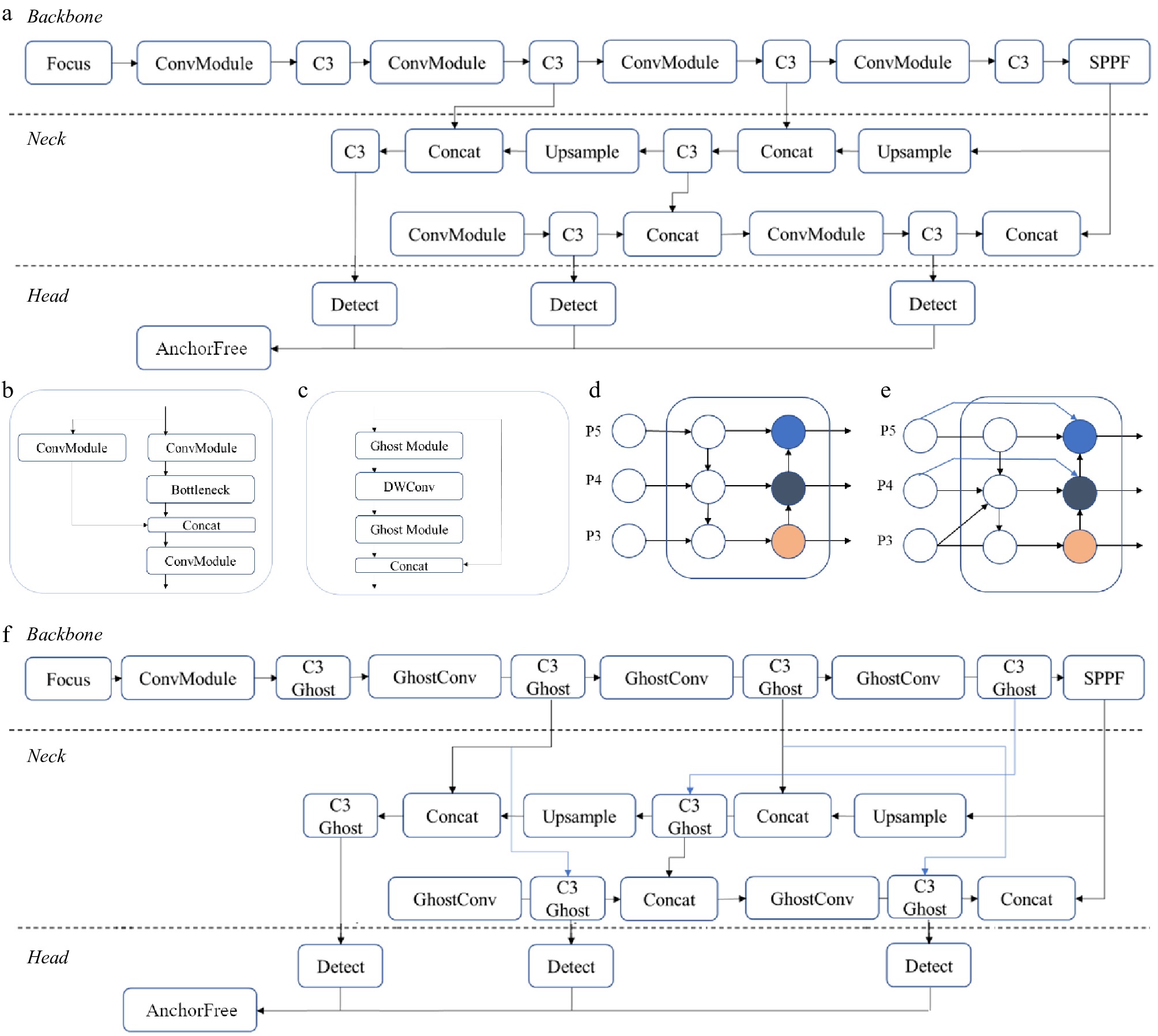
Figure 4. 

YOLOv5 and key modules: a) YOLOv5 architecture b) C3 module; c) Ghost module; d) PANet neck as FPN (top-down path), and PAN (down-top path); e) BiFPN neck; f) modified YOLOv5 architecture.

Modification in the neck network

In this study, the projected blueberry size varied from 0.5 to 4.5 cm², resulting in different interest pixel regions for the detection based on YOLO. The neck network needs to process multiple-scale features generated by the backbone networks. As presented in Fig. 4d, PANet^[23] merged the down-top path aggression network over the Feature Pyramid Network (FPN) with a top-down path aggression^[24]. In the neck network in YOLO, only the formal layers including P3, P4, and P5 were utilized. The PANet, with both top-down and down-top path aggression, could transfer the strong semantic information possessed between deep feature layers. However, there was still a limitation over such architecture, as there might be feature maps missing during the information transformation from the formal structure of PANet with the top-down path aggression. In addressing this challenge, we employed an enhanced bidirectional feature pyramid network^[25] to optimize the existing YOLOv5 neck network. As presented in Fig. 4e, the BiFPN network establishes a bidirectional channel, introduces a cross-scale connection methodology, incorporates an additional edge, and integrates the relative size features from FPN along the bottom-up path. This strategic augmentation aims to refine the overall performance and efficiency of the YOLOv5 architecture, elevating its capabilities in blueberry detection and recognition in this study. The final architecture of the modified YOLOv5 is presented in Fig. 4f.

Training process

For the model training, we selected the YOLOv5, YOLOv8, and YOLOv11 architectures^[20,21] as baseline encompassing distinct configurations including nano, small, medium variants, and modifications of YOLOv5-Ghost, YOLOv5-bifpn, and YOLOv5-Ghost-bifpn. We selected CNN-based object detection models over Vision Transformer (ViT) models for their implicit local feature beneficial for blueberry detection (Supplementary Table S1). The models were trained with the augmented training images at a resolution of 640 × 640 × 3. The total training epoch was set at 300. Additionally, the YOLOv5 input layer incorporated a mosaic data enhancement technique^[21]. This innovative approach involves the fusion of four images by resizing each of them, seamlessly stitching them together, and applying random cutouts within the resultant composite image. The integration of this data enhancement technique within the YOLOv5 framework serves to address data concentration and imbalance issues across small, medium, and large target data, offering a comprehensive solution for more robust object detection.

The training and testing processes were carried out on a desktop with RTX 4070 SUPER 12GB and Ubuntu 20.04 through Windows Subsystem for Linux (WSL) for Windows 11. The models with the best validation performance were exported to TensorFlow Lite files with fp16 quantization for mobile inference and selected as the YOLOv5-based model.

The portrait image was resized and padded horizontally to a 640 × 640 RGB image as the model input. Then Non-Maximum Suppression (NMS) boxes was used to filter for boxes with greater than 50% confidence for blueberry detection. The radius of the inscribed circle was taken for each blueberry NMS box, and the average area of the circles was used to calculate the average blueberry area estimation.

Android application

Both of these methods were integrated into an Android application using the Python Kivy graphics user interface (GUI) framework and tested on a Pixel 7 running Android 12. The application allows users to capture images and choose the method for generating pixel area estimations with the flowchart (Fig. 5). The application will display the image with detected berries and numerical outputs of berry count and size estimate. Given that the radius in the HT method relies on the distance to a sample, the user has the flexibility to fine-tune the model by adjusting radius parameters in the application. These computational outputs were then logged in a CSV file recorded within the device storage including timestamps of each image, details of applied methods, the respective counts, and the calculated average area.

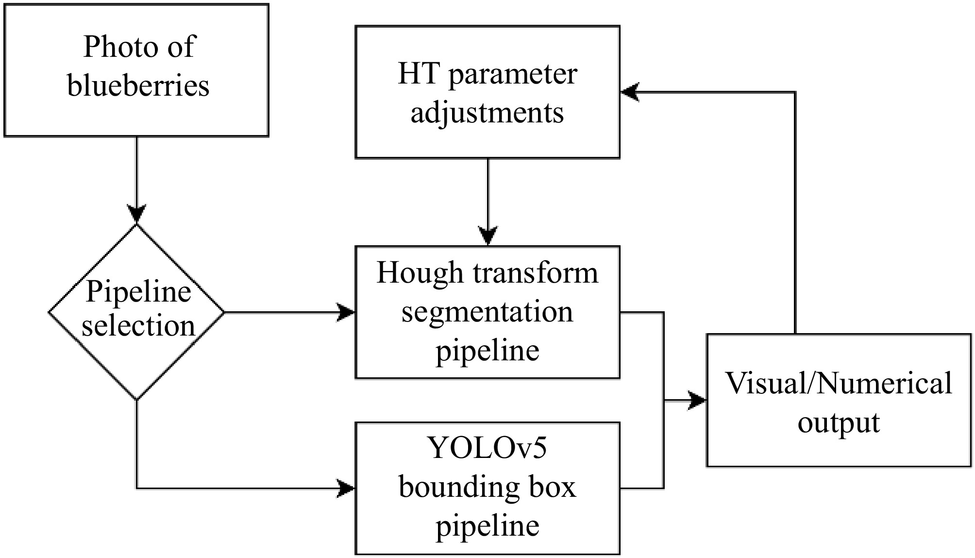
Figure 5. 

Android application flowchart. The user captures an image from the camera, selects a pipeline and obtains the results in a feedback image and recorded CSV entry.

To accommodate varying camera-to-object distances, the application integrated an important feature for distance calibration. This functionality involved utilizing a 5 × 5 checkerboard pattern positioned within the camera's field of view. OpenCV functions were employed to detect the corners of the chessboard, enabling the image to be scaled for a consistent distance of 50 pixels between the corners. This functionality is particularly advantageous in situations where there are varying distances to consider during usage. By implementing this method, the application can autonomously execute the entire image-to-weight estimation algorithm in handheld mode without the need for depth imaging.

Evaluation metrics

The performance of all blueberry detection models was assessed using Precision (P), Recall (R), Average Precision (AP), mean Average Precision (mAP) with an intersection-of-union (IoU), and inference speed, in which mAP was a key metric to evaluate the overall performance of a model. The equations used to calculate these measures are as follows:

where, TP is the number of true positive blueberries detected, FP is the number of false blueberries detected, and FN is the number of blueberries falsely not detected as blueberries; AP_k represents the AP of class k; n represents the number of classes. The IoU threshold was set at 0.5, meaning that the result is true positive if the IoU between the predicted result and ground truth bounding boxes was greater than 0.5.

Image size to real size normalization

Distance between the camera and berries as well as zoom in or out setting on the phone slightly varied between datasets (Supplementary Fig. S3). To ensure a more consistent representation of the model outputs, we performed normalization by converting the area from pixels to cm². This was achieved by measuring pixel-to-cm ratios based on the weighing boat's dimensions as the reference. The ratios were obtained from six manually selected images in the dataset: one from the first dataset, two from the second dataset, and three from the third dataset. These ratios were approximately [98.067, 103.667, 110.80, 116.0, 111.87, 113.67] pixels/cm, respectively, and calculated based on the 15 cm bottom plate edge length. These ratios were applied to their respective categories after obtaining the model estimations.

The results indicate that YOLOv5m achieved the highest mAP among the three models, at 93.5 for mAP_50-95, which were 2.3% and 0.8%, respectively, higher than that of YOLOv5n and YOLOv5s (Table 1). However, as for the inference time based on the computing environment (NVIDIA RTX4070 SUPER) used in this study, YOLOv5m was the slowest and with the heaviest parameter count of 25.0 × 10⁶, compared to the parameter count of 2.50 × 10⁶ for YOLOv5n and 9.11 × 10⁶ for YOLOv5s. For the smartphone application, the YOLOv5s was selected as a baseline model for its balanced performance in mAP_50-95 (92.7%) and inference time (203.4 ms per image), which is 38.2% of YOLOv5m inference time.

The evaluation of modified YOLOv5 models encompasses key metrics including: parameter count, inference time, and mAP₅₀ and mAP_50-95 scores (Table 1). The modified models evaluated in this study are named A, B, and C, with each model undergoing different levels of modification (YOLOv5s + GhostNet, YOLOv5s + biFPN, and YOLOv5s + GhostNet + biFpn).

Count estimation

For blueberry counting, the HT-based method miscounted 51 blueberries out of 4,604 blueberries (1.108%) across the dataset, where 32 out of 198 images (16.162%) had miscounts in them. The YOLOv5-based method miscounted two out of 4,604 blueberries (0.0434%), in two out of 198 images (1.01%) with 0.5 confidence. The miscounts were caused by either extremely small berries or clustered samples with examples shown in Fig. 6a−d.

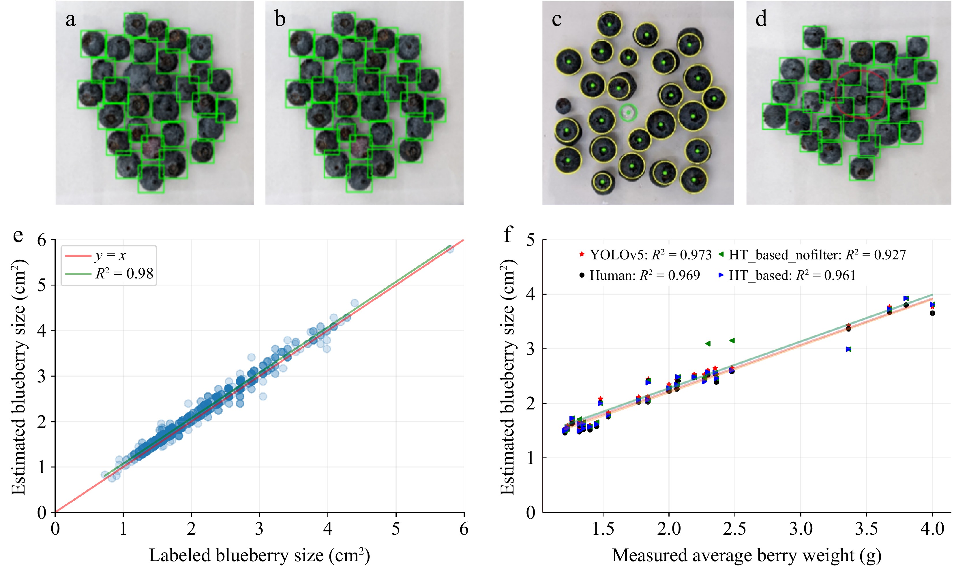
Figure 6. 

Model performances in counting, size estimation, and weight estimation. (a), (b) confidence threshold miscounts for YOLOv5. (c), (d) Miscount examples from both methods. HT-based filtered the green circle but misses the left small blueberry. YOLOv5 failed to detect the red circled blueberry in cluster. (e) Comparison between individual blueberry size estimations by YOLOv5 and manually labeled size estimations for the test set. (f) The correlation between estimated average berry weight (g) and manually measured berry weight (g).

Size estimation

Figure 6e shows the size estimation for individual blueberries in the test set for the YOLOv5-based model. The majority of estimated blueberry sizes highly correlated with annotated berry size with R² = 0.98 (Fig. 6e). The best fit line above the y = x line indicates the estimated size is consistently greater than the human labels, specifically with the slope at 0.999 and offset at 0.0751. The average labeled blueberry size is 2.108 cm² and the estimation size is 2.179 cm². The range for the labeled blueberries is [0.729, 5.792] cm² and the estimation range is [0.751, 5.792] cm².

Weight estimation

Figure 6f shows the pixel-to-centimeter-area normalized model outputs compared to the measured average blueberry weights in grams. All models display a similar linear correlation under a high value of coefficient of determination (R² > 0.96), with the highest R² (0.973) for the YOLOv5-based model. These automated models demonstrated comparable performance in terms of the R² (0.969) between the blueberry area estimated from manually labeled bounding boxes and the measured weight. Size estimations obtained from the average pixel area of the HT-based model with the circularity filter showed a higher R² (0.961) value than without the circularity filter (R² = 0.927), where the data points around x = 2.5 g are better estimated by the filter. We used a linear model to fit the size-to-weight relationship because of the high linear relationship between measured weights and estimated size given by $y_{area}=m\ \times\ y_{weight}+b$. The weight estimation was derived as ${y}_{weight}=({y}_{area}-b)/m$ using the previous equation, where m = [0.859, 0.848, 0.854] and b = [0.550, 0.527, 0.489] for YOLOv5-based, HT-based, and ground truth based on the labeled bounding boxes from the dataset, respectively. The weight estimation percent error, $\mathrm{\%}error=100\ \times\ |y_{measured}-y_{weight}|/y_{measured}$, on average were 6.615%, 5.702%, and 5.843% for the HT-based, YOLOv5-based, and human labels, respectively. The mean absolute error (MAE) for the HT-based and YOLOv5-based models were 0.1249 and 0.0997 g, respectively, while the human label MAE was 0.1038 g for the average berry.

Android application

Figure 7 shows the Android Python application using Kivy with the GUI developed for berry detection and size estimation. We selected four models, YOLOv5n, YOLOv5s, YOLOv5m, and YOLOv5s-C, for mobile inference. The amount of time from image capture to the output on a Pixel 7 was 0.256, 0.521, 1.262, and 0.459 seconds, respectively. The image was taken at a resolution of 640 × 480 pixels as shown in Fig. 7. The parameters for HT-based model were fine-tuned using the GUI feedback through the red and green circles to detect all blueberries. The time required for area estimation was slower for YOLOv5-based model with 1.262 s and 1.023 s for the HT-based model.

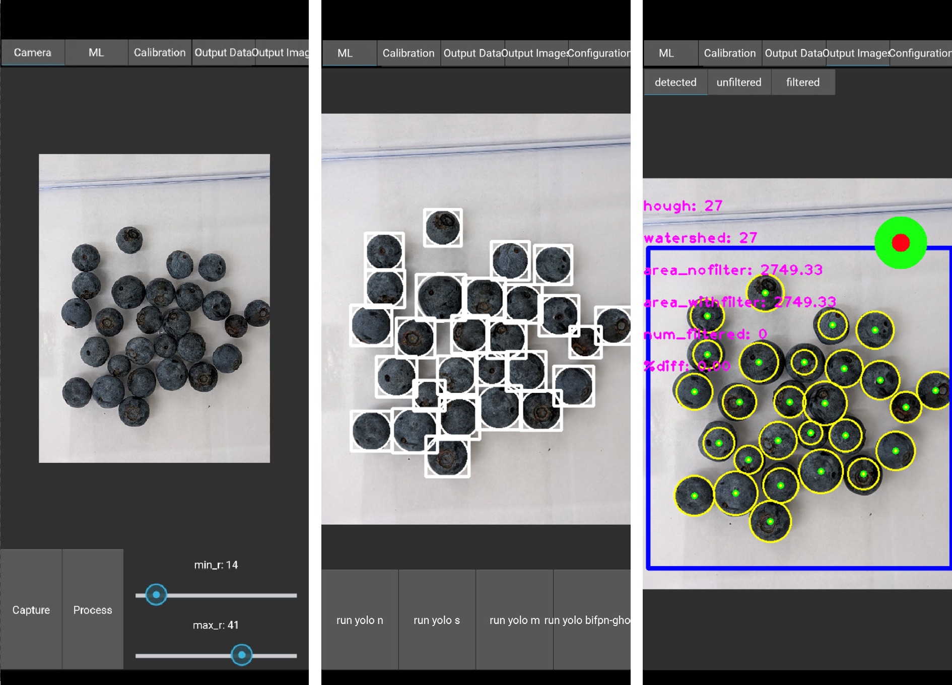
Figure 7. 

Screenshots of the Android application in portrait mode, from left to right: the captured image with radius parameters, the YOLOv5-based detection, and the HT-based detection.

The counting performance of the YOLOv5-based model demonstrates that our method could significantly reduce the need for manual counting and establish a reliable foundation for estimating the average weight. The HT-based model was sensitive to outliers because it filters circles using user-defined radius bounds. The YOLOv5-based model was sensitive to clustered samples because of the overlapping filter parameter in the NMS algorithm.

The YOLOv5s-A model stands out compared to the baseline with a reduced parameter count of 5.77 million and accelerated inference time at 136.0 ms/image, which is 66.9% of the inference time of the original network. As for detection performance, it maintains a 99.4% mAP₅₀ score and 91.6% in mAP_50-95, showcasing its efficiency. Conversely, the model incorporating modified biFPN exhibits a higher parameter count (9.18 × 10⁶) and a slower inference time (202.6 ms/image) but compensates with higher mAP_50-95 score of 92.9%, which is similar with YOLOv5s. The YOLOv5s-C model incorporates both Ghost and biFPN architectures, results in 5.84 million parameters, inference time of 143.5 ms/image, and a mAP_50-95 score of 91.9%. In summary, the C model offers the improvements of both A and B models to the original YOLOv5s, excelling in parameter count and inference time, all while upholding a mAP₅₀ of 99.4% and mAP_50-95 of 91.9% with reduced parameters of 5.84 × 10⁶. Both YOLOv5-based and HT-based models had similar processing times on the Android device. However, the HT-based model's time depends on the number of blueberries due to the complexity of HT and watershed algorithms, while the YOLOv5-based model's inference time remains consistent across different scenarios.

YOLO series algorithms have been applied to various agricultural counting tasks, such as corn stand counting, apple detection and counting^[26], and strawberry yield estimation^[27]. For example, YOLOv3-tiny has been used to count corn plants at different growth stages, achieving high accuracy rates of over 98% in certain conditions, but it can struggle with overlapping plants at later growth stages^[28]​. Similarly, YOLO has proven effective for dense object detection, such as counting soybean pods, where YOLO POD^[29], a specialized variant, was developed to handle the dense and overlapping nature of pods​.

In our study, we observed R² = 0.98 from the best performing model in blueberry size estimation to manually labeled sizes and R² = 0.973 between blueberry size and weight. The high correlation (r = 0.986) in our study was supported by previous studies. Mengist et al.^[8] compared manually measured berry weight and image-based berry volume measurements of 54 blueberry accessions, with a minimum of 10 berries per accession. Results showed that fruit weight was highly correlated with fruit volume (p < 0.001, r = 0.99). A strong and significant correlation between berry weight and diameter was also reported among 58 southern highbush cultivars (R² = 0.94)^[30]. This strong correlation between berry size and weight enables researchers to phenotype only one trait while predicting the other.

Much of the previous research has focused on model performance rather than the practical deployment on mobile devices or embedded systems, which are crucial for real-time field applications. In contrast, the lightweight algorithm developed in this study is optimized for such platforms, enabling efficient deployment on resource-constrained devices like smartphones and edge computing units. With minimal modifications, it can be easily adapted to other counting tasks, such as fruit yield estimation or plant disease detection, offering a flexible solution across various agricultural scenarios.

The application offers several advantages over the manual process of counting and weighing blueberry samples across different genotypes and datasets. Instead of manually counting and weighing berries, users can simply take images of the berries to obtain an accurate estimation of berry size and use berry size to estimate berry weight. In addition, users can also weigh a handful of berries and use image-based analysis to detect berry counts and automatically calculate berry weight. As a result, this tool can: (1) significantly reduce the labor and time cost of blueberry size and weight phenotyping; and (2) provide additional information on variation of berry size and weight.

Limitations and future research

This study was conducted using datasets gathered in a controlled environment, therefore the application may underperform in conditions involving significant changes in lighting, background, and berry display, as noted in outdoor studies^{[13,14,16,17]}. In our future research, we plan to collect datasets in dynamic environments, aiming to train the models under varied conditions and thereby enhance the application's overall robustness. To further fortify the adaptability of these models across diverse breeding and research programs, an in-depth exploration into a broader range of datasets becomes imperative. Incorporating datasets that encapsulate various environmental factors, genetic variations, and phenotypic traits is critical to ensuring the models' versatility and efficacy across a spectrum of applications.

Future Android application development should prioritize enhancing the GUI design and integrating additional features, such as the capability to import and export images and incorporating built-in weight estimation instead of pixel area-based weight estimation. Using a more industry-standard development platform, such as Android Studio in Java, would contribute to a more polished application. Furthermore, it is necessary to assess the performance of the models across various breeding programs and phenotyping platforms to enhance their robustness and user-friendliness.

We assessed the inference speed performance on a Pixel 7 device, with each model processing every image in less than one second, thereby making it possible to count the blueberries and estimate weight faster than the manual process. The processing time can be potentially further reduced by using pruned YOLO models or downsampled images, although this may result in slightly less accurate estimations.

Counting and weighing blueberries manually is a repetitive and time-consuming task, yet it remains crucial for blueberry breeding, research, and production. To automate this process, we integrated computer vision and machine learning techniques implemented on embedded platforms. In this research, we developed two different approaches for blueberry counting, sizing, and weight estimation in controlled environments. Specifically, one approach relies on conventional computer vision techniques where the Hough Transform was implemented to detect individual blueberries, while the other employs deep learning models where modified YOLOv5-based models (YOLOv5s + Ghost + biFPN) were trained for blueberry detection and segmentation with reduced size and parameters. Both models demonstrated high performance in terms of counting accuracy and weight estimation, which is comparable to human labeling. They achieved 99.85% counting accuracy and showed a highly linear relationship (R² > 0.96) between pixel area size and measured weight, with an MAE less than 0.10 g and an average error of less than 6%. Area-based estimation proved to be more reliable than other models utilizing count-based weight estimations, as many images contain equal berry counts but very different berry weights.