Exploring a cost-effective way for nutrient management with machine learning for container plants

Container plant production for indoor and patio uses, including ornamental plants, vegetables, and herbs, has become an important segment of green industry. Precision irrigation and fertilization schedules for container crops have been developed and widely used for nursery stocks and gardening^[1]. However, several problems related to nutrient deficiency and excessiveness due to the improper use of water-soluble fertilizer, failed rate control of slow-release fertilizer, and untimely and abrupt heavy irrigation, could lead to significant reductions in plant health with lower foliar and floral qualities, causing economic waste, eutrophication, and environmental pollution^[2]. Over the past century, a tremendous amount of fertilizer, especially anthropogenic nitrogen (N) fertilizer, in the amount of 100 TgN·yr⁻¹, has been applied to agricultural systems^[3,4]. Considering plants can only absorb 35% of the applied fertilizer, even under ideal conditions, and N fertilizer costs experienced significant inflation in the past 5 years by increasing 150%^[5], an improved fertilizer use efficiency with precise fertilization scheduling is desired for container plant production. To provide timely references for restoring or cutting-off fertilizer supply, it is essential to monitor and track changes in plant nutrient conditions, which could provide insights into the current status of fertilization input rate.

Direct accurate and timely measurements of plant nutrient concentrations require time-consuming and labor-intensive sample collection and lab analysis, which is normally destructive and site-specific for the plant. The direct relationships between leaf chlorophyll content and tissue N concentration, along with the absorption or reflectance of different light wavelengths (e.g., red, blue) due to the presence of chlorophyll, has fostered the development of indirect fast and non-destructive methods for detecting N concentrations, these methods utilize optical meters or reflectance sensors and can be applied at the whole-plant level^[6,7]. Studies have tested the use of red–green–blue (RGB), fluorescence, multispectral, and hyperspectral imaging systems to estimate plant leaf or whole-plant N nutrient levels or chlorophyll content in vegetable, floriculture, and agronomy crops^[8−10]. However, limited access, difficulty in selecting appropriate imaging systems, and the high costs of cameras or sensors restrict growers' ability to fully adopt these technologies^[11]. To improve the accessibility of these technologies, several studies have developed cost effective imaging systems to detect plant N or stress status: Adhikari et al.^[7] used low-cost RGB camera (with light filters) to detect the reflectance ratio of red and near infrared light from poinsettia (Euphorbia pulcherrima), which resulted in a well-fitted regression with chlorophyll concentration and tissues N contents; Kamarianakis & Panagiotakis^[12] created an affordable chlorophyll meter that uses light-to-voltage measurements to assess the residual light after two light emitting diode (LED) emissions pass through a brussels sprouts (Brassica oleracea) leaf, which had a high correlation with Soil Plant Analysis Development (SPAD) meter values; Legendre et al.^[13] used an RGB camera to capture Madagascar periwinkle (Catharanthus roseus images) under blue LEDs with a bandpass filter (650–740 nm) as a chlorophyll fluorescence imaging system to detect plant stress responses, which has the potential to be used in detecting N stress. Most of these studies used simple regression analysis to quantify the continuous (or numerical) values, but this approach can be challenging for growers to interpret, as their primary concern is whether fertilizer levels are insufficient or sufficient. Applying supervised machine learning with both regression for continuous values and classification for discrete categories to determine nutrient status and provide references for fertilization guidance (underuse or overuse) at the whole-plant level can address this limitation^[14]. Additionally, a wide range of testing studies for container crops, including vegetables, herbs, and ornamentals are less reported. Therefore, the objectives of this study are: 1) evaluate the stability of a cost-effective RGB imaging system for detecting plant nutrient status of four types of container crops, quantify and correlate plant growth with imaging values; 2) find decision-making thresholds for fertilization based on different fertilizer input rates; and 3) find machine learning algorithms with higher accuracy to guide fertilization schedules of the container plants.

This study was conducted in a greenhouse located at the University of Georgia-Griffin Campus (33.26° N, 84.28° W, Griffin, GA, USA) during the summer of 2023. Environmental conditions inside the greenhouse were controlled using a WADSWORTH Control System (EnviroSTEP; Arvada, CO, USA) and monitored with a suite of sensors: a temperature and humidity sensor (HMP60; Vaisala, Vantaa, Finland) and a light sensor (SQ-618 ePAR; Apogee Instruments, Logan, UT, USA), both were connected to a datalogger (CR1000X; Campbell Scientific, Logan, UT, USA). During the study period (8 weeks), the daily average temperature, relative humidity, vapor pressure deficit, and daily light integral were 26.4 ± 1.4 °C, 71.7 ± 8.1%, 0.97 ± 0.28 kPa, and 30.62 ± 5.98 mol·m^–2·d^–1, respectively.

Plant material, growth conditions, and treatment factors

Four types of container plants were used to conduct the study: pepper (Capsicum annuum, cv. 'Capperino'), basil (Ocimum basilicum, cv. 'Cinnamon'), marigold (Tagetes patula, cv. 'Queen Sophia'), and sage (Salvia officinalis). All seeds (Johnny's Selected Seeds, Winslow, ME, USA) were seeded (three seeds per pot) into nursery pots (15 cm top diameter × 14 cm height) filled with peat-based growth media (Pro-mix, Quakertown, PA, USA). Overhead irrigation was regularly applied without any fertilization. After 3 weeks of growth, seedlings were thinned to one to keep the plants uniform. Five levels of weekly fertilizer input treatments based on N rates (0%, 25%, 50%, 75%, and 100% of full rate) were initiated to impose on the plants for 4 weeks (Table 1) with each pot receiving 250 mL nutrient solution. The recommended 100% fertilizer input rate for container plants were adjusted from Schwarz et al.^[15]. For each type of crop, each treatment level was assigned randomly to five pots, with fertilization applied using 20–20–20 (N–P–K) water-soluble fertilizer (Peters Professional, OH, USA). The study was arranged with a completely randomized design for each crop. Routine management practices were performed during the experimental period including daily irrigation, pest control using yellow sticky traps, and weed control by hand weeding.

Plant images and growth measurements

An overhead imaging system was established using an RGB camera (EOS Rebel T7; Cannon, Melville, NY, USA) mounted on a tripod (NEEWER, Shenzhen, China) positioned at a height of 1.5 m. During the 4-week study period (plant vegetative growth stage), weekly images were taken of each crop and treatment over a total of 11 d, with each image captured on a randomly selected day within the week (0, 3, 8, 9, 10, 14, 15, 16, 17, 23, and 24 d after treatment began), and a known-area square (red, 3 cm × 3 cm) was used as a reference. After taking the images, ImageJ^[16,17] was used to automatically establish thresholds using color histogram to segment out the plant canopy from the background, targeted mask (plant canopy) was then used to calculate canopy area and perform automatic pipeline color analysis by separating the image into different color spaces to calculate the average red, green, and blue values (Fig. 1). Plant height, two perpendicular widths, and leaf chlorophyll content averaged from three mature leaves quantified by a SPAD meter (SPAD-502; Konica Minolta, Ramsey, NJ, USA) were measured weekly. Growth index (GI) was calculated using the formula: GI = (Height + (Width1 + Width2)/2)/4^[18]. At the end of the experiment, plant dry weight (DW) was measured after oven drying for 3 d at 80 °C.

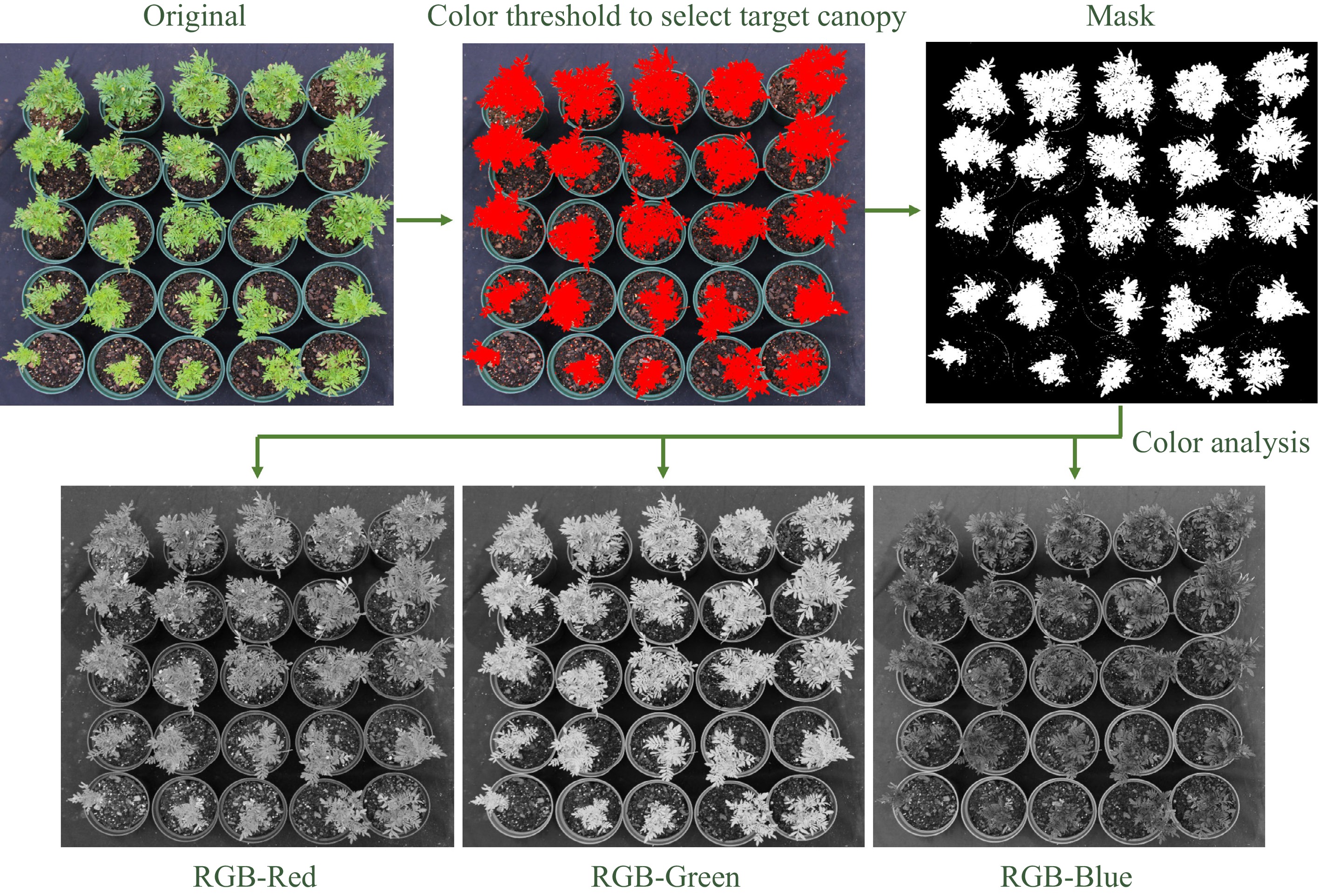
Figure 1. 

Illustration of image analysis flowchart with an example of marigold plants. Color thresholds were established to segment out the plant canopy from the background, targeted mask (plant canopy) was then used to calculate canopy area and perform color analysis by separating the image into different color spaces (red, green, and blue).

Statistical analysis and machine learning approaches

This experiment was conducted in a completely randomized design for each crop with five treatment factors (Nrate1–Nrate5) and five replications. Data were analyzed using R^[19] and one-way analysis of variance (ANOVA) was used to test the effects of fertilization levels on plant growth and development changes. When the main effect was significant, the mean comparison was conducted using Tukey's honest significant difference (HSD) test at 5% probability. Values of canopy area (CA), red (R), green (G), and blue (B) from images, and leaf chlorophyll content (LCC), growth index (GI), and dry weight (DW) as indicators of plant nutrient status were analyzed to assess their correlations (Pearson correlation) and similarities were categorized across fertilizer input levels. This enabled the creation of four fertilization guidance categories from the treatments based on their similarity from cluster analysis: extreme-underuse (plants had extremely stunned growth), sub-underuse (plants had reduced growth), sufficient use (plants had normal growth), and overuse (plants growth was not improved even with improved fertilizer input). After labeling all the fertilization categories, five supervised machine learning models (k nearest neighbor, KNN; decision tree, DT; random forest, RF; support vector machine, SVM; naïve Bayes, NB) were compared to find the best algorithms with the highest classification accuracy using the image data (canopy area and RGB values). R packages kknn, Rpart, randomForest, e1071, naivebayes were used for model evaluation, specifically, for each model test, the total data size was 25 (5 replication × 5 treatments), 70% of the image data (data set size 17 was separated using seed 123 in R, Supplementary File 1) was used to train the algorithms and the remaining 30% data (data size 8) was used to test and calculate the identification accuracy. To ensure robust analysis, data distribution was checked with variances, data distribution histograms and boxplots, and was found to not be suffering from extreme skewness or outliers with balanced and normal distribution; we also checked the overfitting concerns using cross-validation (e.g., k-fold cross-validation), the accuracies from the cross-validation were higher or closer to the training data, indicating there was low presence of the overfitting problem.

Our RGB imaging system successfully identified the objectives of plant canopy for all types of crops, and automatically calculated the canopy areas and color values for individual plants under five fertilization treatment levels. Image analysis showed that differences in canopy area expansion were detectable as early as one week after treatments began. In contrast, reductions in canopy color values were observed over the growth period, with treatment-related differences in color, especially red and green values, becoming distinguishable only at later stages (Supplementary Figs S1–S4). For basil, increased fertilization positively affected canopy red and green color values, while the opposite trend was observed for marigold and pepper; sage canopy color values, however, showed no significant response to fertilization rates. All the types of crops exhibited remarkable increases in leaf chlorophyll content, canopy area, growth index, and dry weight due to the increased fertilization input (Table 2).

Clustering similar treatments for new fertilization input levels

Among the five fertilization input rates during the plant vegetative growth stage, basil, marigold, pepper, and sage plants all showed similar responses within the nearby rates (e.g., Nrate4 and Nrate5), indicating that higher fertilizer inputs may be redundant if the lower input rates produce comparable plant growth. Using similarity analysis, we grouped fertilization inputs with similar plant responses by clustering them closely based on the Euclidean distances calculated from the measured parameters. For basil, Nrate4 and Nrate5-treated plants had similar growth with higher growth index, dry weight, canopy area, leaf chlorophyll content, and canopy red and green values compared to other rates, indicating Nrate5 was an overuse rate (plant growth was not improved even with improved fertilizer input) and Nrate4 was a sufficient rate (plants had normal growth) to meet plant demand; while Nrate3 was a sub-underuse rate (plants had reduced growth), Nrate1 and Nrate2 were extreme-underuse rates (plants had extremely stunned growth) since they were clustered together. Basil canopy development and biomass showed strong positive correlations among each other, and color values derived from image analysis were also positively correlated with plant growth parameters, except that canopy color values were not significantly correlated with leaf chlorophyll content (Fig. 2a, b). Marigold, pepper, and sage exhibited trends similar to basil, with Nrate5 as an overuse level, Nrate4 as a sufficient level, Nrate3 as a sub-underuse level, Nrate1 and Nrate2 as extreme-underuse levels. Growth parameters for these plants were positively correlated with each other. However, unlike basil, canopy red and green values of marigold and pepper were negatively correlated with their growth parameters including leaf chlorophyll content (Fig. 2c–h).

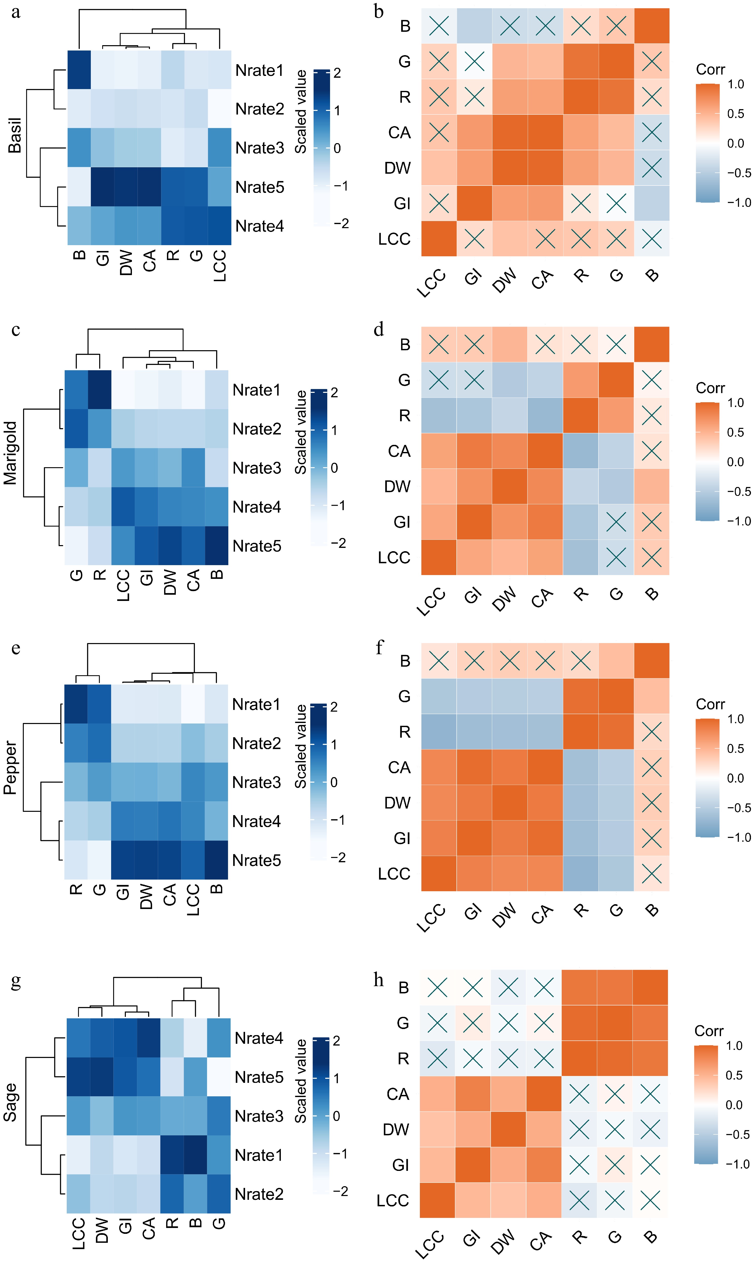
Figure 2. 

Heatmaps with clustering, and correlograms of (a), (b) basil, (c), (d) marigold, (e), (f) pepper, and (g), (h) sage for plant leaf chlorophyll content (LCC), growth index (GI), dry weight (DW), and canopy area (CA), red (R), green (G), blue (B) values from image analysis as affected by different fertilization input treatments based on N rates (Nrate1, 2, 3, 4, 5). For heatmaps with clustering, each row represents a treatment, and each column represents a measured variable. All data are standardized, and measured variables are clustered based on their correlations. For correlograms, Pearson correlation coefficient (r) values are used to calculate the strength (basis of judgment) and direction of a linear relationship between two variables, p-values based on the calculated r value and sample size (n) using a t-distribution with (n-2) degrees of freedom is used to indicate statistically significant correlations. X indicates insignificant correlation coefficients (p ≥ 0.05).

Testing accuracy for machine learning models

Based on the plant nutrient status indicated by the measured parameters, fertilization input rates were labeled with meaningful guidance categories: extreme-underuse, sub-underuse, sufficient use, and overuse. Five supervised machine learning models using image analysis data were then evaluated for their accuracy in classifying plant nutrient status due to different fertilizer inputs during the plant vegetative growth stage (Fig. 3). Results showed that identification accuracy reached up to 0.8 for basil using KNN and SVM, 0.7 for marigold using KNN and Naïve Bayes, 0.9–1.0 for pepper using KNN and SVM, and 0.7 for sage using Naïve Bayes. Additionally, accuracy improved significantly after two weeks of treatment, with peak accuracy occurring between three and four weeks after treatment started.

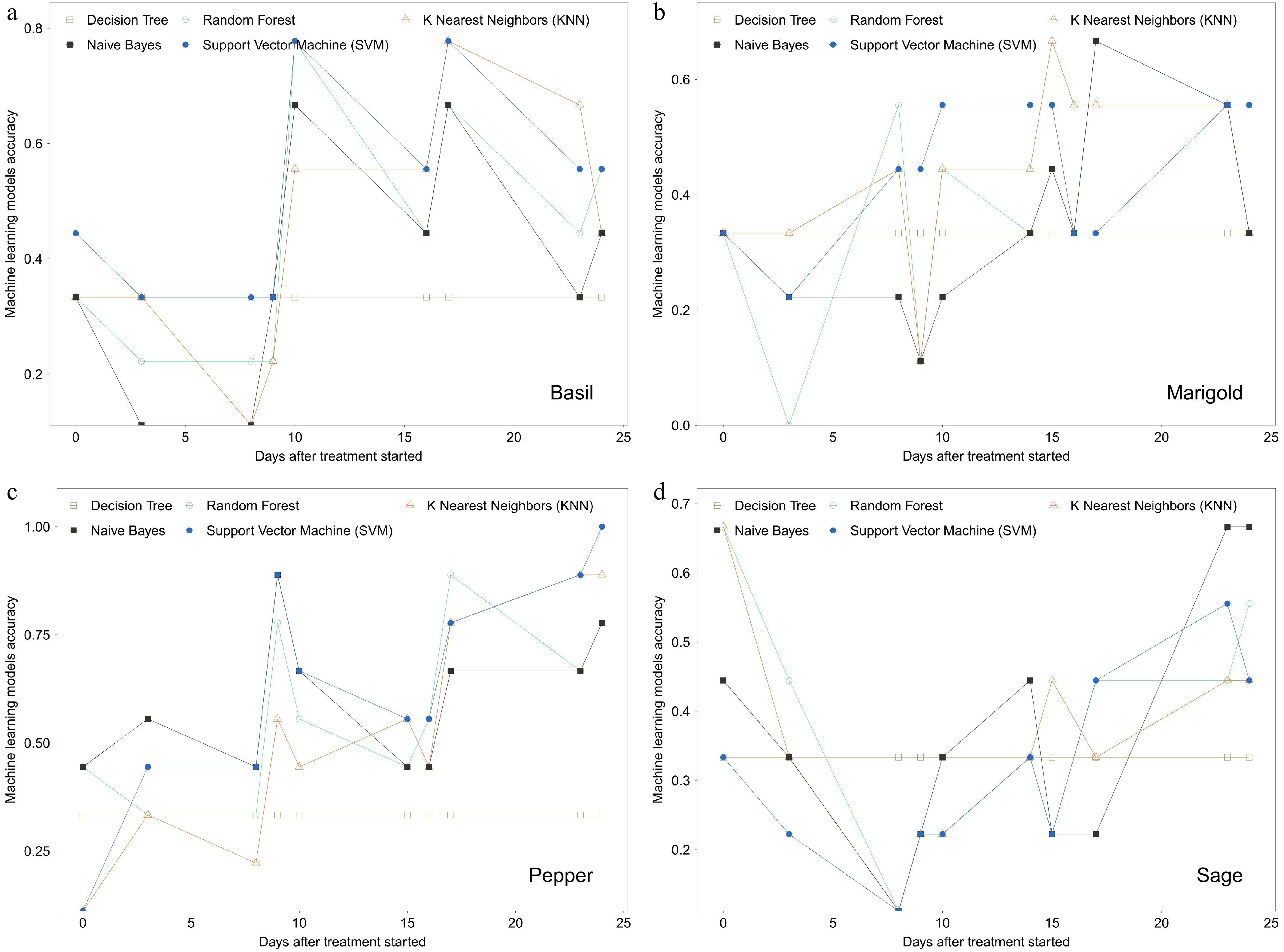
Figure 3. 

Machine learning model accuracy evaluation for four fertilization status labeled based on clustering (extreme-underuse, sub-underuse, sufficient use, and overuse) of (a) basil, (b) marigold, (c) pepper, and (d) sage. Training and testing data contain only canopy area, red, green, and blue values from image analysis.

Fertilization input directly affects plant growth performance, as shown in our study results. The highest fertilization input based on nitrogen (Nrate5) had doubled biomass accumulation in basil and sage, and tripled in marigold and pepper, as compared with the lowest rate (Nrate1). Leaf chlorophyll content, as an important indicator for plant nutrient conditions, was significantly affected by fertilizer rates in all the container crops. The differences in fertilization input could also be detected from image analysis-derived data, such as canopy area, and red and green color values.

Detecting nutrient status under variable fertilization rates using image analysis to guide nutrient management has become increasingly efficient and accurate. This technique was tested mostly in agronomy crops, where imaging systems could remotely obtain plant greenness index and RGB color values, and correlated these numbers with actual nitrogen concentration in maize (Zea mays) or chlorophyll content in sorghum (Sorghum bicolor) to identify the under-input rate of fertilization^[9,20]. However, simple regression analysis sometimes resulted in lower coefficients of determination (R² = 0.6 – 0.8). Researchers started to use conventional machine learning algorithms (SVM, KNN, decision tree) and even deep learning approaches (convolutional neural network) to identify plant nutrient status from RGB images, such as identifying nitrogen stress levels (healthy, semi stressed, and severely stressed) in sorghum (Sorghum bicolor) and maize (Zea mays), which could reach up to 0.91 and 0.97 accuracies with the potential to guide the nutrient management^[14,21]. In recent years, vegetable and ornamental crops have been introduced to test the efficacy of the combination use of image analysis and prediction models: 0.2–0.8 coefficients of determination were obtained using a conventional machine learning model to predict aquaponic lettuce (Lactuca sativa) leaf chlorophyll content using RGB values^[22]; 0.38–0.84 coefficients of determination were achieved using regression model to predict poinsettia (Euphorbia pulcherrima) tissue N content using multispectral values^[10]. Our study, a comprehensive evaluation of various container crops including vegetables, ornamentals, and herbs, demonstrated that using an RGB imaging system could effectively monitor the growth conditions of basil, marigold, pepper, and sage. The strong correlations between the image data and plant growth measurements further justified the use of the system. The system provided accurate guidance for fertilization schedules with 0.7–1.0 accuracy in identifying whether the fertilization levels were deficient, sufficient, or excessive during the plant's vegetative growth stage. Machine learning models, such as KNN, SVM, and Naïve Bayes, have proved their effectiveness in assisting nutrient management of container crops along with the imaging system. Moreover, RF typically needs a larger sample size to generate reliable and generalizable results, but for this study, we included RF only for comparing with other traditional machine learning models. Due to the limitations, future studies with increased sample size are required to create reliable and informative RF results.

Unlike conventional approaches, that only used color values from imaging techniques to assess or predict plant nutrient status^[23], our study incorporated canopy area, derived from image analysis, to enhance fertilization guidance, as canopy area showed to be a strong factor in affecting the accuracy of machine learning-based identification. However, we found the accuracy was low during the first two weeks of treatment, indicating the delayed detection from the system. It could be because when plants were young, they were less susceptible to nutrient stress. Although average accuracy improved gradually each week, it remained inconsistent at shorter intervals, especially when assessed over 2- to 3-d periods. This could be caused by light variations on those days, which could affect the color values derived from image analysis. For the consideration of practical use in container plant production, we recommend using a color panel as a reference to standardize color values derived from image analysis.

In our study, we used plant leaf chlorophyll content (SPAD), growth index, biomass, canopy area, and RGB colors derived from image analysis as indicators to indicate plant vigorous and to cluster the similarities of the fertilization treatments. SPAD had been widely measured to identify fertilization input levels (especially based on nitrogen) and was positively correlated with plant biomass and yield^[24]. Plant growth index, biomass, and leaf area were directly affected by fertilization levels, which were normally separated by extremely low to excessive fertilization input rates according to common nursery usage rate^[25]. For clarity and to enhance our machine learning analysis, we labeled the treatments as 'underuse', 'sufficient', or 'excessive', these categories are specific to our study; in practical applications, growers may need to adjust these classifications based on other target outcomes (e.g., nutrient use efficiency, yield, or dry weight). We acknowledge that our selected parameters did not cover all aspects of plant development. Future work will include additional measurements—such as photosynthetic rate, chlorophyll fluorescence, and nutrient uptake efficiency—to achieve a more comprehensive assessment of fertilizer impact.

Overall, building the imaging system cost approximately USD${\$}$500, with 90% of the cost attributed to the camera. By replacing RGB camera modules connected with small single-board computers (e.g., Raspberry Pi), the cost could be reduced to around USD${\$}$150^[7].

This study tested container plants (basil, marigold, pepper, and sage) growth responses to five fertilization input rates based on nitrogen during the plant vegetative growth stage, and found that plant chlorophyll content, growth index, canopy area, and biomass were gradually increased along with increased fertilizer rates. We built an RGB imaging system with a supervised machine learning approach to track plant canopy development and identify fertilization input status (deficient, sufficient, or excessive) due to the close correlations between the image data and plant growth measurements. The system could provide 0.7–1.0 accuracy in guiding fertilization schedules using KNN, SVM, and Naïve Bayes models after 3 weeks of treatment during the plant vegetative growth stage. Cluster analysis proved to be a promising approach for identifying fertilization status for plant nutrient management. This imaging system could offer a cost-effective and real-time monitoring for precision nutrient management, and potentially be used as a decision-making control platform based on identified fertilization input status to increase profits by reducing the cost of excessive fertilizer input and expenses associated with human errors, reduce environmental pollution from substantial fertilizer leaching in container crop production, and benefit long-term fertilizer use efficiency.